We have explored disturbance rejection in the gravity drained tanks process using P-Only and then PI control. In the PI study, we confirmed the observations we had made in the PI control of the heat exchanger investigation.
In particular, we learned that PI controllers:
▪ can eliminate the offset associated with P-Only control,
▪ have integral action that increases the tendency for the PV to roll (or oscillate),
▪ have two tuning parameters that interact, making it challenging to correct tuning when performance is not acceptable.
Here we investigate the benefits and challenges of derivative action and PID control when disturbance rejection remains our control objective.’
As with all controller implementations, we follow our four-step design and tuning recipe. A benefit of this recipe is that steps 1-3 are independent of the controller used, so our previous results from steps 1 and 2 (detailed here) and step 3 (detailed here andhere) can be used in this PID study.
We summarize those previous results before proceeding to step 4 and the design and tuning of a PID controller (nomenclature for this article is listed in step 4).
Step 1: Determine the Design Level of Operation (DLO)
The control objective is to reject disturbances as we control liquid level in the lower tank. Our DLO for this study is:
▪ design PV and SP = 2.2 m with range of 2.0 to 2.4 m
▪ design D = 2 L/min with occasional spikes up to 5 L/min
Step 2: Collect Process Data around the DLO
When CO, PV and D are steady near the design level of operation (DLO), we bump the CO as detailed here and force a clear response in the PV that dominates the noise.
Step 3: Fit a FOPDT Model to the Dynamic Process Data
We approximate the dynamic behavior of the process by fitting test data with a first order plus dead time (FOPDT) dynamic model. A fit of step test data and doublet test data yields these values:
▪ process gain (how far), Kp = 0.09 m/%
▪ time constant (how fast), Tp = 1.4 min
▪ dead time (how much delay), Өp = 0.5 min
Step 4: Use the FOPDT Parameters to Complete the Design
The preferred PID algorithm in industrial practice employs derivative on PV, and vendors market this controller in several different forms. Each algorithm form has its own tuning correlations, and if we take care to match algorithm with correlation, they all provide identical capability and performance.
For tuning, we rely on the industry-proven Internal Model Control (IMC) tuning correlations. These require only one specification, the closed loop time constant (Tc), that describes the desired speed or quickness of our controller in responding to a set point (SP) change or rejecting a disturbance (D).
Our PI control study describes what to expect from an aggressive, moderate or conservative controller. Once our desired performance is chosen, the closed loop time constant is computed:
▪ aggressive: Tc is the larger of 0.1·Tp or 0.8·Өp
▪ moderate: Tc is the larger of 1·Tp or 8·Өp
▪ conservative: Tc is the larger of 10·Tp or 80·Өp
Because the popular PID forms perform the same if properly tuned, the observations and conclusions we draw from any one algorithms applies to the other forms.
Dependent Ideal PID
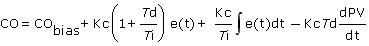
Among the most widely used algorithms is the Dependent Ideal (Non-interacting) PID form:
![]()
Where:
CO = controller output signal (the wire out)
CObias = controller bias; set by bumpless transfer
e(t) = current controller error, defined as SP – PV
SP = set point
PV = measured process variable (the wire in)
Kc = controller gain, a tuning parameter
Ti = reset time, a tuning parameter
Td = derivative time, a tuning parameter
• Design and Tune
In the P-Only study, we had established that for the gravity drained tanks process:
▪ sample time, T = 1 sec
▪ the controller is reverse acting
▪ dead time is small compared to Tp and thus not a concern in the design
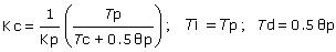
After we choose a Tc based on our desired performance, the tuning correlations for the Dependent Ideal PID form are:
Similar to the PI controller tuning correlations, only controller gain contains Tc, and thus, only Kc changes based on the need for a more or less active controller.
• Implement and Test
We first explore an aggressive response tuning for our ideal PID controller:
Aggressive Tc = the larger of 0.1·Tp or 0.8·Өp
= larger of 0.1 (1.4 min) or 0.8 (0.5 min)
= 0.4 min
Using this Tc and our Kp, Tp and Өp from Step 3 in the tuning correlations above, we compute these aggressive controller gain, reset time and derivative time tuning values:
Aggressive Ideal PID: Kc = 28 %/m; Ti = 1.7 min; Td = 0.21 min
The performance of this controller in rejecting changes in the pumped flow disturbance (D) for the gravity drained tanks is shown to the right in plot below (click for a large view). For comparison, the performance of an aggressive PI controller is shown in the plot to the left (design details here). Note that the set point (SP) remains constant at 2.2 m throughout the study.
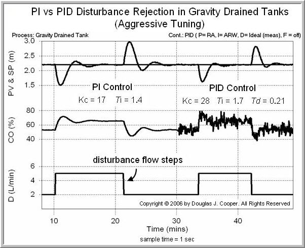
The maximum deviation of the PV from set point during the disturbance rejection event is smaller for the PID controller relative to the PI controller. The PID controller also provides a faster settling time because derivative action tends to reduce the rolling or oscillatory behavior in the PV trace.
Like the heat exchanger PID study, there is an obvious difference in the CO signal trace for the PI vs PID controllers. Derivative action causes the noise (random error) in the PV signal to be amplified and reflected in the control output (CO) signal.
Such extreme control action will cause excessive wear in a valve or other mechanical final control element, requiring increased maintenance. This consequence of noise in the measured PV can be a serious disadvantage with PID control.
Ideal vs Interacting PID
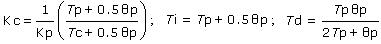
We compare the Dependent Ideal PID form above to the performance of the Dependent Interacting PID form and establish that they are identical in performance if properly tuned. The Dependent Interacting form is written:
• Design and Tune
We use the same rules above to choose a Tc that reflects our desired performance. The IMC tuning correlations for the Dependent, Interacting form are then:
As before, only controller gain contains Tc, and thus, only Kc changes based on a desire for a more or less active controller. Sample time remains for this implementation at T = 1 sec and the controller remains as reverse acting.
• Implement and Test
We choose a moderate response tuning in this example:
Moderate Tc = the larger of 1·Tp or 8·Өp
= larger of 1.0 (1.4 min) or 8 (0.5 min)
= 0.4 min
Using this Tc and our model parameters in the proper tuning correlations (ideal or interacting), we arrive at these moderate tuning values:
Moderate Ideal PID: Kc = 4.3 %/m; Ti = 1.7 min; Td = 0.21 min
Moderate Interacting PID: Kc = 3.7 %/m; Ti = 1.4 min; Td = 0.25 min
As shown in the plot below (click for a large view), moderate tuning provides a reasonably fast disturbance rejection response while producing little or no oscillations as the PV settles.
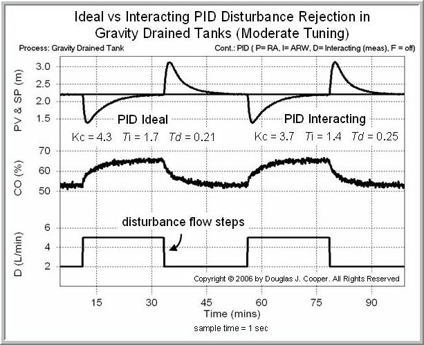
The indistinguishable behavior confirms that the two controllers indeed are identical in capability and performance if tuned with their own correlations.
| Aside: Our observations using the dependent ideal and dependent interacting PID algorithms directly apply to the other popular PID controller forms. For example, the independent PID algorithm form is written: 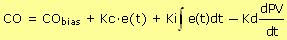 The integral and derivative gains in the above independent form can be computed, for example, using the ideal PID correlations as: Ki = Kc/Ti and Kd = Kc×Td. Because of these mathematical identities, performance and capability observations drawn about one algorithm will apply directly to the other. |
Ideal Moderate vs Ideal Aggressive
As shown in the plot below (click for a large view), we compare moderate tuning side-by-side with aggressive tuning for the dependent ideal PID controller. For a different perspective, we make this comparison using a set point tracking objective.
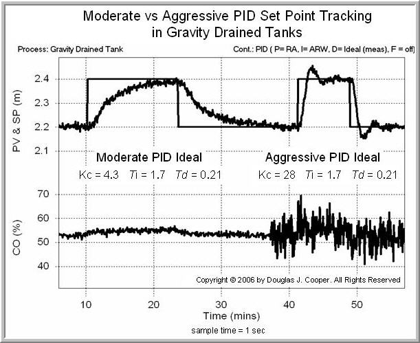
The performance of the two controllers matches the design descriptions provided here. That is, a controller tuned with:
▪ a moderate Tc will move the PV reasonably fast while producing little to no overshoot.
▪ an aggressive Tc will move the PV quickly enough to produce some overshoot and then oscillation as the PV settles out.
Need for CO Filtering
The excessive activity in the CO signal can be a problem, and a controller output (CO)signal filter is one solution. An interesting observation from the above plot is that the degree of “chatter” in the CO signal grows as controller gain, Kc, increases.