We have explored the open loop (manual mode) operation and behavior of the gravity drained tanks process and have worked through the first two steps of the controller design and tuning recipe.

As those articles discuss:
 ▪ Our measured process variable, PV, is liquid level in the lower tank,
 ▪ The set point, SP, is held constant during normal production operation,
 ▪ Our primary control challenge is rejecting unexpected disruptions from D, the pumped flow disturbance.

We have generated process data from both a step test and a doublet test around our design level of operation (DLO), which for this study is:

 ▪ Design PV and SP = 2.2 m with range of 2.0 to 2.4 m
 ▪ Design D = 2 L/min with occasional spikes up to 5 L/min

Here we present step 3 of our recipe and focus on a graphical analysis of the step test data. Next we will explore modeling of the doublet test data using software.

Data Accuracy
We should understand that real plant data is rarely as perfect as that shown in the plots below. As such, we should not seek to extract more information from our data than it actually contains.

In the analyses presented here, we display extra decimals of accuracy only because we will be comparing different modeling methods over several articles. The extra accuracy will help when we make side-by-side comparisons of the results.

Step 3: Fit a FOPDT Model to the Data
The third step of the recipe is to describe the overall dynamic behavior of the process with an approximating first order plus dead time (FOPDT) dynamic model.

We will move quickly through the graphical analysis of step response data as we already presented details of the procedure in the heat exchanger study.

• Process Gain – The “How Far” Variable
Process gain, Kp, describes how far the PV moves in response to a change in controller output (CO). It is computed:

where DPV and DCO represent the total change from initial to final steady state. The path or length of time the PV takes to get to its new steady state does not enter into the Kp calculation.

Reading the numbers off of our step test plot below (click for a large view), the CO was stepped from a steady value of 55% down to 51%.

The PV was initially steady at 2.38 m, and in response to the CO step, moved down to a new steady value of 2.02 m.

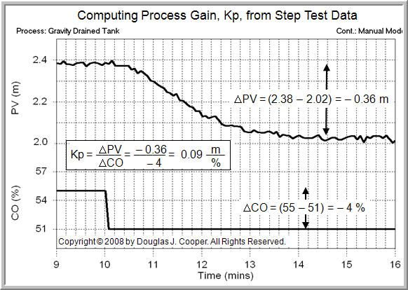
Using these in the Kp equation above, the process gain for the gravity drained tanks process around a DLO (design level of operation) PV of about 2.2 m when the pumped disturbance (not shown in the plot) is constant at 2 L/min is:

For further discussion and details, the process gain calculation for the heat exchanger step test is presented here.

• Time Constant - The “How Fast” Variable
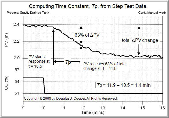
The time constant, Tp, describes how fast the PV moves in response to a change in the CO.

For step test data, Tp can be computed as the time that passes from when the PV shows its first response to the CO step, until when the PV reaches 63% of the total DPV change that is going to occur.

The time constant must be positive and have units of time. For controllers used on processes comprised of gases, liquids, powders, slurries and melts, Tp most often has units of minutes or seconds.

For step test data, we compute Tp in five steps (see plot below):
  1. Determine DPV, the total change in PV from final steady state minus initial steady state
  2. Compute the value of the PV that is 63% of the way toward the total DPV change, or “initial steady state + 0.63(DPV)”
  3. Note the time when the PV passes through the “initial steady state + 0.63(DPV)” value
  4. Subtract from it the time when the “PV starts a first clear response” to the step change in the CO
  5. The passage of time from step 4 minus step 3 is the process time constant, Tp.

Following the procedure for the plot above (click for a large view):

 1. The PV was initially steady at 2.38 m and moved to a final steady state of 2.02m. The total change, DPV, is “final minus initial steady state” or:
     DPV = 2.02 – 2.38 = –0.36 m

 2. The value of the PV that is 63% of the way toward this total change is “initial steady state + 0.63(DPV)” or:
     Initial PV + 0.63(DPV) = 2.38 + 0.63(–0.36)
                                   = 2.38 – 0.23
                                   = 2.15 m

 3. The time when the PV passes through the “initial steady state PV + 0.63(DPV)” point of 2.15 m is:
     Time to 0.63(DPV) = Time to 2.15
                              = 11.9 min

 4. The time when the “PV starts a first response” to the CO step is:
     Time PV response starts = 10.5 min

 5. The time constant is “time to 63%(DPV)” minus “time PV response starts” or:
     Tp = 11.9 – 10.5 = 1.4 min

There are further details and discussion on the process time constant and its calculation from step test data in the heat exchanger example presented in another article.

• Dead Time - The “How Much Delay” Variable
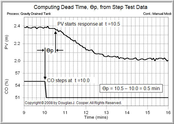
Dead time, Өp, is the time delay that passes from when a CO action is made and the measured PV shows its first clear response to that action.

Like a time constant, dead time has units of time, must always be positive, and for processes with streams comprised of gasses, liquids, powders, slurries and melts, is most often expressed in minutes or seconds.

Estimating dead time, Өp, from step test data is a three step procedure:
  1. Locate the time when the “PV starts a first clear response” to the step change in the CO. We already identified this point when we computed Tp above.
  2. Locate the point in time when the CO was stepped from its original value to its new value.
  3. Dead time, Өp, is the difference in time of step 1 minus step 2.

Applying this procedure to the step test plot above (click for a large view):

 1. As identified in the plot above, the PV starts a first clear response to the CO step at 10.5 min (this is the same point we identified in the Tp analysis),

 2. The CO step occurred at 10.0 min, and thus,

 3. Өp = 10.0 – 10.5 = 0.5 min

Additional details and discussion on process dead time and its calculation from step test data can be found in the heat exchanger example presented here.

Note on Units
During a dynamic analysis study, it is best practice to express Tp and Өp in the same units (e.g. both in minutes or both in seconds). The tuning correlations and design rules assume consistent units.

Also, the process gain, Kp, should be expressed in the same (though inverse) units of the controller gain, Kc, (or proportional band, PB) used by our manufacturer.

Control is challenging enough without adding computational error to our problems.

Validating Our FOPDT Model
It is good practice to validate our FOPDT model before proceeding with design and tuning. If our model describes the dynamic data, and the data is reflective of the process behavior, then the last step of the recipe follows smoothly.

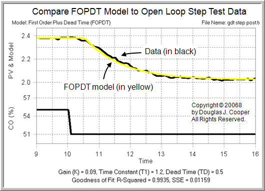
The FOPDT model parameters we computed from the analysis of the step test data are:
  ▪ Process gain (how far), Kp = 0.09 m/%
  ▪ Time constant (how fast), Tp = 1.4 min
  ▪ Dead time (how much delay), Өp = 0.5 min

Recall that, using the nomenclature of this site, the FOPDT dynamic model has the general form:

And this means that the dynamic behavior of the gravity drained tanks can be reasonably approximated around our DLO as:

Where: t [=] min, PV [=] m, CO [=] %

The plot below (click for large view) compares step test data from the gravity drained tanks process to this FOPDT model.

Visual inspection confirms that the simple FOPDT model provides a very good approximation for the behavior of this process.

Specifically, our graphical analysis tells us that for the gravity drained tanks process, with a DLO PV of about 2.2 m when the pumped disturbance is constant at 2 L/min:
  ▪ the direction PV moves given a change in CO
  ▪ how far PV ultimately travels for a given change in CO
  ▪ How fast PV moves as it heads toward its new steady state
  ▪ how much delay occurs between when CO changes and PV first begins to respond

This is precisely the information we need to proceed with confidence to step 4 of the design and tuning recipe.

Modeling Doublet Test Data
We had suggested in a previous article that a doublet test offers benefits as an open loop method for generating dynamic process data. These include that the process:
  ▪ starts from and quickly returns to the DLO,
  ▪ yields data both above and below the design level to “average out” the nonlinear effects, and
  ▪ the PV always stays close to the DLO, thus minimizing off-spec production.

We next explore using commercial software to fit a FOPDT model to doublet test data. Return to the Table of Contents to learn more.