Like the P-Only controller, the Proportional-Integral (PI) algorithm computes and transmits a controller output (CO) signal every sample time, T, to the final control element (e.g., valve, variable speed pump). The computed CO from the PI algorithm is influenced by the controller tuning parameters and the controller error, e(t).
PI controllers have two tuning parameters to adjust. While this makes them more challenging to tune than a P-Only controller, they are not as complex as the three parameter PID controller.
Integral action enables PI controllers to eliminate offset, a major weakness of a P-only controller. Thus, PI controllers provide a balance of complexity and capability that makes them by far the most widely used algorithm in process control applications.
The PI Algorithm
While different vendors cast what is essentially the same algorithm in different forms, here we explore what is variously described as the dependent, ideal, continuous, position form:
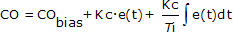
Where:
CO = controller output signal (the wire out)
CObias = controller bias or null value; set by bumpless transfer as explained below
e(t) = current controller error, defined as SP – PV
SP = set point
PV = measured process variable (the wire in)
Kc = controller gain, a tuning parameter
Ti = reset time, a tuning parameter
The first two terms to the right of the equal sign are identical to the P-Only controller referenced at the top of this article.
The integral mode of the controller is the last term of the equation. Its function is to integrate or continually sum the controller error, e(t), over time.
Some things we should know about the reset time tuning parameter, Ti:
| ▪ | It provides a separate weight to the integral term so the influence of integral action can be independently adjusted. |
| ▪ | It is in the denominator so smaller values provide a larger weight to (i.e. increase the influence of) the integral term. |
| ▪ | It has units of time so it is always positive. |
Function of the Proportional Term
As with the P-Only controller, the proportional term of the PI controller, Kc·e(t), adds or subtracts from CObias based on the size of controller error e(t) at each time t.
As e(t) grows or shrinks, the amount added to CObias grows or shrinks immediately and proportionately. The past history and current trajectory of the controller error have no influence on the proportional term computation.
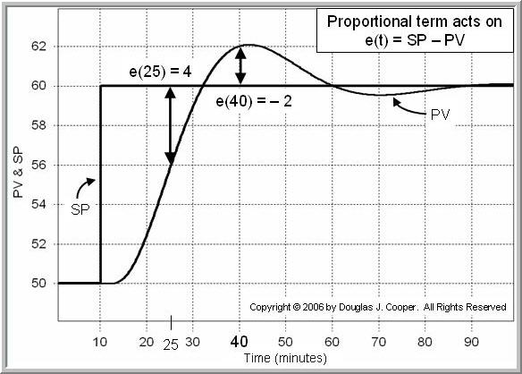
The plot below (click for a large view) illustrates this idea for a set point response. The error used in the proportional calculation is shown on the plot:
▪ At time t = 25 min, e(25) = 60–56 = 4
▪ At time t = 40 min, e(40) = 60–62 = –2
Recalling that controller error e(t) = SP – PV, rather than viewing PV and SP as separate traces as we do above, we can compute and plot e(t) at each point in time t.
Below (click for a large view) is the identical data to that above only it is recast as a plot of e(t) itself. Notice that in the plot above, PV = SP = 50 for the first 10 min, while in the error plot below, e(t) = 0 for the same time period.

This plot is useful as it helps us visualize how controller error continually changes size and sign as time passes.
Function of the Integral Term
While the proportional term considers the current size of e(t) only at the time of the controller calculation, the integral term considers the history of the error, or how long and how far the measured process variable has been from the set point over time.
Integration is a continual summing. Integration of error over time means that we sum up the complete controller error history up to the present time, starting from when the controller was first switched to automatic.
Controller error is e(t) = SP – PV. In the plot below (click for a large view), the integral sum of error is computed as the shaded areas between the SP and PV traces.

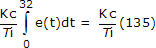
Each box in the plot has an integral sum of 20 (2 high by 10 wide). If we count the number of boxes (including fractions of boxes) contained in the shaded areas, we can compute the integral sum of error.
So when the PV first crosses the set point at around t = 32, the integral sum has grown to about 135. We write the integral term of the PI controller as:
Since it is controller error that drives the calculation, we get a direct view the situation from a controller error plot as shown below (click for a large view):

Note that the integral of each shaded portion has the same sign as the error. Since the integral sum starts accumulating when the controller is first put in automatic, the total integral sum grows as long as e(t) is positive and shrinks when it is negative.
At time t = 60 min on the plots, the integral sum is 135 – 34 = 101. The response is largely settled out at t = 90 min, and the integral sum is then 135 – 34 + 7 = 108.
Integral Action Eliminates Offset
The previous sentence makes a subtle yet very important observation. The response is largely complete at time t = 90 min, yet the integral sum of all error is not zero.
In this example, the integral sum has a final or residual value of 108. It is this residual value that enables integral action of the PI controller to eliminate offset.
As discussed in a previous article, most processes under P-only control experience offset during normal operation. Offset is a sustained value for controller error (i.e., PV does not equal SP at steady state).
We recognize from the P-Only controller:
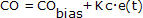
that CO will always equal CObias unless we add or subtract something from it.
The only way we have something to add or subtract from CObias in the P-Only equation above is if e(t) is not zero. It e(t) is not steady at zero, then PV does not equal SP and we have offset.
However, with the PI controller:
we now know that the integral sum of error can have a final or residual value after a response is complete. This is important because it means that e(t) can be zero, yet we can still have something to add or subtract from CObias to form the final controller output, CO.
So as long as there is any error (as long as e(t) is not zero), the integral term will grow or shrink in size to impact CO. The changes in CO will only cease when PV equals SP (when e(t) = 0) for a sustained period of time.
At that point, the integral term can have a residual value as just discussed. This residual value from integration, when added to CObias, essentially creates a new overall bias value that corresponds to the new level of operation.
In effect, integral action continually resets the bias value to eliminate offset as operating level changes.
Challenges of PI Control
There are challenges in employing the PI algorithm:
| ▪ | The two tuning parameters interact with each other and their influence must be balanced by the designer. |
| ▪ | The integral term tends to increase the oscillatory or rolling behavior of the process response. |
Because the two tuning parameters interact with each other, it can be challenging to arrive at “best” tuning values. The value and importance of our design and tuning recipeincreases as the controller becomes more complex.
Initializing the Controller for Bumpless Transfer
When we switch any controller from manual mode to automatic (from open loop to closed loop), we want the result to be uneventful. That is, we do not want the switchover to cause abrupt control actions that impact or disrupt our process
We achieve this desired outcome at switchover by initializing the controller integral sum of error to zero. Also, the set point and controller bias value are initialized by setting:
▪ SP equal to the current PV
▪ CObias equal to the current CO
With the integral sum of error set to zero, there is nothing to add or subtract from CObias that would cause a sudden change in the current controller output. With the set point equal to the measured process variable, there is no error to drive a change in our CO. And with the controller bias set to our current CO value, we are prepared by default to maintain current operation.
Thus, when we switch from manual mode to automatic, we have “bumpless transfer” with no surprises. This is a result everyone appreciates.
Reset Time Versus Reset Rate
Different vendors cast their control algorithms in slightly different forms. Some use proportional band rather than controller gain. Also, some use reset rate, Tr, instead of reset time. These are simply the inverse of each other:
Tr = 1/Ti
No matter how the tuning parameters are expressed, the PI algorithms are all equally capable.
But it is critical to know your manufacturer before you start tuning your controller because parameter values must be matched to your particular algorithm form.Commercial software for controller design and tuning will automatically address this problem for you.
Implementing a PI controller
We explore PI controller design, tuning and implementation on the heat exchanger in this article and the gravity drained tanks in this article.