In a previous article, we looked at the structure of the P-Only algorithm and we considered some design issues associated with implementation. We also studied the set point tracking (or servo) performance of this simple controller for the heat exchangerprocess.
Here we investigate the capabilities of the P-Only controller for liquid level control of the gravity drained tanks process. Our objective in this study is disturbance rejection (or regulatory control) performance.
Gravity Drained Tanks Process
A graphic of the gravity drained tanks process is shown below (click for a large view):
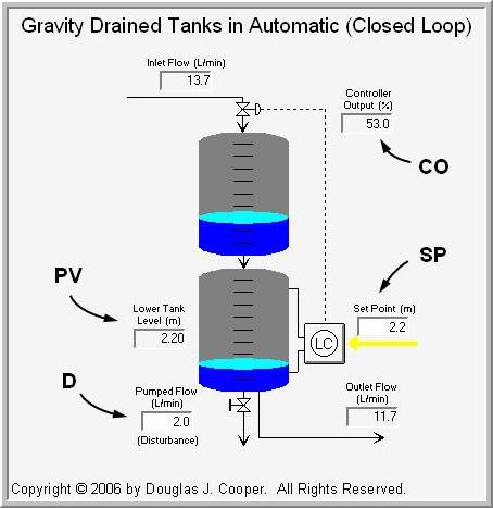
The measured process variable (PV) is liquid level in the lower tank. The controller output (CO) adjusts the flow into the upper tank to maintain the PV at set point (SP).
The disturbance (D) is a pumped flow out of the lower tank. It’s draw rate is adjusted by a different process and is thus beyond our control. Because it runs through a pump, D is not affected by liquid level, though the pumped flow rate drops to zero if the tank empties.
We begin by summarizing the previously discussed results of steps 1 through 3 of ourdesign and tuning recipe as we proceed with our P-Only control investigation:
Step 1: Determine the Design Level of Operation (DLO)
Our primary objective is to reject disturbances as we control liquid level in the lower tank. As discussed here, our design level of operation (DLO) for this study is:
▪ design PV and SP = 2.2 m with range of 2.0 to 2.4 m
▪ design D = 2 L/min with occasional spikes up to 5 L/min
Step 2: Collect Process Data around the DLO
When CO, PV and D are steady near the design level of operation, we bump the CO far enough and fast enough to force a clear dynamic response in the PV that dominates the signal and process noise. As detailed here, we performed two different open loop (manual mode) dynamic tests, a step test and a doublet test.
Step 3: Fit a FOPDT Model to the Dynamic Process Data
The third step of the recipe is to describe the overall dynamic behavior of the process with an approximating first order plus dead time (FOPDT) dynamic model. We define the model parameters and present details of the model fit of step test data here. A model fit of doublet test data using commercial software confirms these values:
▪ process gain (how far), Kp = 0.09 m/%
▪ time constant (how fast), Tp = 1.4 min
▪ dead time (how much delay), Өp = 0.5 min
Step 4: Use the FOPDT Parameters to Complete the Design
Following the heat exchanger P-Only study, the P-Only control algorithm computes a CO action every loop sample time T as:
CO = CObias + Kc∙e(t)
Where:
CObias = controller bias or null value
Kc = controller gain, a tuning parameter
e(t) = controller error, defined as SP – PV
· Sample Time, T
Best practice is to set the loop sample time, T, at one-tenth the time constant or faster (i.e., T ≤ 0.1Tp). Faster sampling may provide modestly improved performance. Slower sampling can lead to significantly degraded performance.
In this study, T ≤ (0.1)(1.4 min), so T should be 8 seconds or less. We meet this specification with the common vendor sample time option:
▪ sample time, T = 1 sec
· Control Action (Direct/Reverse)
The gravity drained tanks has a positive Kp. That is, when CO increases, PV increases in response. When in automatic mode (closed loop), if the PV is too high, the controller must decrease the CO to correct the error (read more here). Since the controller must move in the direction opposite of the problem, we specify:
▪ controller is reverse acting
· Dead Time Issues
If dead time is greater than the process time constant (Өp > Tp), control becomes increasingly problematic and a Smith predictor can offer benefit. For this process, the dead time is smaller than the time constant, so:
▪ dead time is small and thus not a concern
· Computing Controller Error, e(t)
Set point, SP, is manually entered into a controller. The measured PV comes from the sensor (our wire in). Since SP and PV are known values, then at every loop sample time, T, controller error can be directly computed as:
▪ error, e(t) = SP – PV
· Determining Bias Value, CObias
CObias is the value of CO that, in manual mode, causes the PV to remain steady at the DLO when the major disturbances are quiet and at their normal or expected values. Ourdoublet plots establish that when CO is at 53%, the PV is steady at the design value of 2.2 m, thus:
▪ controller bias, CObias = 53%
· Controller Gain, Kc
For the simple P-Only controller form, we use the integral of time-weighted absolute error (ITAE) tuning correlation:
| Moderate P-Only: | 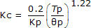 |
| Aside: Regardless of the values computed in the FOPDT fit, best practice is to setӨp no smaller than sample time, T (or Өp ≥ T) in the control rules and correlations (more discussion here). In this gravity drained tanks study, our FOPDT fit produced a Өp much larger than T, so the “dead time greater than sample time” rule is met. |
Using our FOPDT model values from step 3, we compute:

And our moderate P-Only controller becomes:
▪ P-Only controller: CO = 53% + 8∙e(t)
Implement and Test
To explore how controller gain impacts P-Only performance, we test the controller with the above Kc = 8 %/m. Since the correlation tends to produce moderate performance values, we also explore increasingly aggressive or active P-Only tuning by doubling Kc (2Kc = 16 %/m) and then doubling it again (4Kc = 32 %/m).
The ability of the P-Only controller to reject step changes in the pumped flow disturbance, D, is pictured below (click for a large view) for the ITAE value of Kc and its multiples. Note that the set point remains constant at 2.2 m throughout the study.
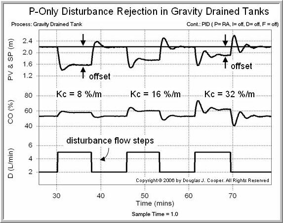
As shown in the figure above, whenever the pumped flow disturbance, D, is at the design level of 2 L/min (e.g., when time is less than 30 min) then PV equals SP.
The three times that D is stepped away from the DLO, however, the PV shifts away from the set point. The simple P-Only controller is not able to eliminate this “offset,” or sustained error between the PV and SP. This behavior reinforces that both set point and disturbances contribute to defining the design level of operation for a process.
The figure shows that as Kc increases across the plot:
▪ the activity of the controller output, CO, increases,
▪ the offset (difference between SP and final PV) decreases, and
▪ the oscillatory nature of the response increases.
Offset, or the sustained error between SP and PV when the process moves away from the DLO, is a big disadvantage of P-Only control. Yet there are appropriate uses for this simple controller (more discussion here).
While not our design objective, presented below is the set point tracking ability of the controller (click for a large view) when the disturbance flow is held constant:
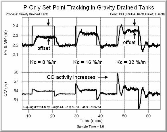
The figure shows that as Kc increases across the plot, the same performance observations made above apply here: the activity of CO increases, the offset decreases, and the oscillatory nature of the response increases.
| Aside: it may appear that the random noise in the PV measurement signal is different in the two plots above, but it is indeed the same. Note that the span of the PV axis in the two plots differs by a factor of four. The narrow span of the set point tracking plot greatly magnifies the signal traces, making the noise more visible. |
Proportional Band
Different manufacturers use different forms for the same tuning parameter. The popular alternative to controller gain found in the marketplace is proportional band, PB.
If the CO and PV have units of percent and both can range from 0 to 100%, then the conversion between controller gain and proportional band is:
PB = 100/Kc
Thus, as Kc increases, PB decreases. This reverse thinking can challenge our intuition when switching among manufacturers.
Many examples on this site assign engineering units to the measured PV because plant software has made the task of unit conversions straightforward. If this is true in your plant, take care when using this formula.
Integral Action
Integral action has the benefit of eliminating offset but presents greater design challenges.