We have discussed the general proportional only (P-Only) algorithm structure and considered important design and tuning issues associated with implementation.
Here we investigate the capabilities of the P-Only controller on our heat exchanger process and highlight some key features and weaknesses of this simple algorithm.
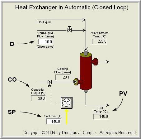
The heat exchanger process used in this study is shown below (click for a large view) and discussed in more detail here.
As with all controller implementations, best practice is to follow the four-step design and tuning recipe as we proceed with the study:
Step 1: Design Level of Operation (DLO)
Real processes display a nonlinear behavior. That is, their process gain (Kp), time constant (Tp) and/or dead time (Өp) changes as operating level changes and as major disturbances change. Since the rules and correlations we use are based on these Kp, Tp and Өp values, controllers should be designed and tuned for a specific level of operation.
The first step in the controller design recipe is to specify our design level of operation (DLO). This includes stating where we expect the set point, SP, and measured process variable, PV, to be during normal operation. Hopefully, these will be the same values as this is the point of a controller.
We also should have some sense of the range of values the SP and PV might assume so we can explore the nature of the process dynamics across that range.
For the heat exchanger, we specify that the SP and PV will normally be at 138 °C, and during production, they may range from 138 to 140 °C. Thus, we can state:
▪ Design PV and SP = 138 °C with range of 138 to 140 °C
We also should know normal or typical values for our major disturbances and be reasonably confident that they are quiet so we may proceed with a bump test. As shown in the graphic above, the heat exchanger process has only one major disturbance variable (D), a side stream labeled Warm Liquid Flow. We specify that the expected or design value for this stream is:
▪ Expected warm liquid flow disturbance, D = 10 L/min
We assume that D remains quiet and at this normal design value throughout the study.
Step 2: Collect Data at the DLO
The next step in the design recipe is to collect dynamic process data as near as practical to our design level of operation. We have previously collected and documentedheat exchanger step test data that matches our design conditions.
Step 3: Fit an FOPDT Model to the Design Data
Here we document a first order plus dead time (FOPDT) model approximation of the heat exchanger step test data from step 2:
▪ Process gain (how far), Kp = – 0.53 °C/%
▪ Time constant (how fast), Tp = 1.3 min
▪ Dead time (how much delay), Өp = 0.8 min
Step 4: Use the Parameters to Complete the Design
The P-Only controller computes a controller output (CO) action every loop sample time T as:
CO = CObias + Kc∙e(t)
Where:
CObias = controller bias or null value
Kc = controller gain, a tuning parameter
e(t) = controller error defined as SP – PV
• Computing controller error, e(t)
Set point (SP) is something we enter into the controller. The PV measurement comes from our sensor (our wire in). With SP and PV values known, controller error can be computed at every loop sample time T as: e(t) = SP – PV.
• Determining Bias Value
CObias is the value of the CO that, in manual mode, causes the PV to steady at the DLO while the major disturbances are quiet and at their normal or expected values.
The plot below (click for a large view) shows that CObias can be located with an ordered search. That is, we move CO up and down while in manual mode until the PV settles at the design value of 138 °C while the major disturbances (trace not shown) are quiet and at their normal or expected values.
Such a manipulation of our process may be impractical or impossible in production situations. The plot is useful, however, because it helps us visualize how the baseline (bias) value of the CO is linked to the design PV.
When we explore PI control of the heat exchanger, we will discuss how commercial controllers use a bumpless transfer method to automatically provide a value for CObias.

The plot above shows that when CO is held constant at 43% with the disturbances at their normal values, the PV steadies at the design value of 138 °C. Thus:
▪ CObias = 43%
• Computing Controller Gain
For the simple P-Only controller, we compute Kc with the integral of time-weighted absolute error (ITAE) tuning correlation:
| Moderate P-Only: | 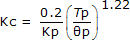 |
This correlation is useful in that it reliably yields a moderate Kc value.
| Aside: Dead time, Өp, is in the denominator in the correlation, so it cannot equal zero. Otherwise, Kc will approach infinity, a fairly useless result.Consider that all controllers measure, act, then wait until next sample time before measuring again. This “measure, act, wait” procedure has a delay (or dead time) of one sample time, T, built naturally into its structure.Thus, by definition, the minimum dead time (Өp,min) in a control loop is the loop sample time, T. Dead time can certainly be larger than sample time and it usually is, but it cannot be smaller.
Whether by software or graphical analysis, if we compute a Өp that is less than T, we must set Өp = T everywhere in our tuning correlations. More information about the importance of sample time to controller design and tuning can be found in this other article. ® Best Practice Rule: |
Using our FOPDT model values from step 3, we compute:
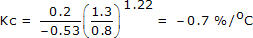
And our moderate P-Only controller becomes:
▪ CO = 43% – 0.7·e(t)
Implement and Test
To explore how controller gain, Kc, impacts P-Only controller behavior, we test the controller with this ITAE controller gain value. Since the Kc value tends to be moderate, we also study more active or aggressive controller behavior when we double Kc and then double it again:
▪ 2Kc = – 1.4 %/°C
▪ 4Kc = – 2.8 %/°C
The performance of the P-Only controller in tracking set point changes is pictured below (click for a large view) for the ITAE Kc and its multiples. Note that the warm liquid disturbance flow, though not shown, remains constant at 10 L/min throughout the study.
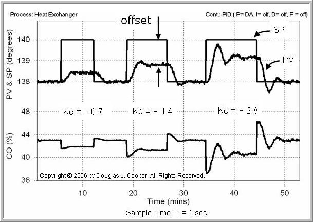
As shown in the figure, whenever the set point is at the design level of 138 °C, then PV equals SP.
Each of the three times the SP is stepped away from the DLO, however, the PV settles out at a value short of the set point. The simple P-Only controller is not able to eliminate this “offset,” or sustained error between the PV and SP. We talk more about offset below.
• Kc and Controller Activity
The plot above shows the performance of the P-Only controller using three different values of Kc.
One point of this study is to highlight that as Kc increases, the activity of the controller output, CO, increases. The CO trace at the bottom of the plot shows this increasingly active behavior, seen as more dramatic moves in response to the same set point step, as Kc increases across the plot.
Thus, we establish that controller gain, Kc, is responsible for the general, and especially the initial, activity in a controller response. This “response activity related to Kc” behavior carries over to PI and PID controllers.
We also see that as Kc increases across the plot, the offset (difference between SP and final PV) decreases but the oscillatory nature of the response increases.
Offset – The Big Disadvantage of P-Only Control
The biggest advantage of P-Only control is that there is only one tuning parameter to adjust, so it is relatively easy to achieve a “best” final tuning. The disadvantage is that this simple control algorithm permits offset.
Offset occurs in most processes under P-Only control when the set point and/or disturbances are at any value other than that used to determine CObias.
To understand why offset occurs, let’s work our way through the P-Only equation:
CO = 43% – 0.7·e(t)
and recognize that:
▪ when PV equals SP, then error is zero: e(t) = 0
▪ if e(t) is zero, then CO equals the CObias value of 43%
▪ if CO is steady at 43%, then the PV settles to 138 °C. We know this is true because that’s how CObias was determined in the first place. The first plot in this article shows us this.
Continuing our reasoning:
▪ the only way CO can be different from the CObias value of 43% is if something is added or subtracted from the 43%
▪ the only way we have something to add or subtract from the 43% is if the error e(t) is not zero
▪ if e(t) is not zero, then PV cannot equal SP, and we have offset.
Possible Applications?
If P-Only controllers permit offset, do they have any place in the process world? Actually, yes.
One example is a surge or swing tank designed to smooth flows between two units. It does not matter what specific liquid level the tank maintains. The level can be at 63% or 36% and we are happy. Just as long as the tank never empties completely or fills so much that it overflows.
A P-Only controller can serve this function. Put the set point at a level of 50% and let the offset happen. We can have the controller implemented quickly and keep it tuned with little effort.