Over a series of articles, we generated step test data from a heat exchanger process simulation and then explored details of how to perform a graphical analysis of the plot data to compute values for a first order plus dead time (FOPDT) dynamic model.
The claim has been that the parameters from this FOPDT model will offer us a good approximation of the complex dynamic behavior of our process. And this, in turn, will provide us information critical for the design and tuning of a PID controller.
So appropriate questions at this point might be:
 How well does our FOPDT model fit the heat exchanger data?
How does this help us design and tune our PID controller?
Comparing Graphical Model to Data
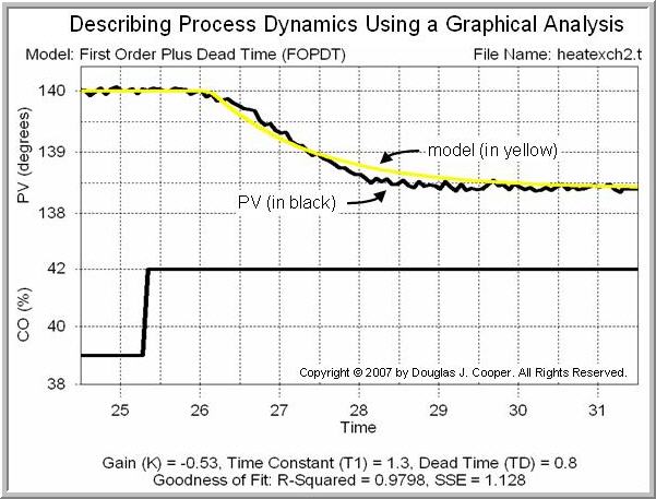
Here are the FOPDT model parameter estimates we computed from the graphical analysis of the step test data (each variable provides a link back to the article with details):
Process gain (how far), Kp = – 0.53 °C/%
Time constant (how fast), Tp = 1.3 min
Dead time (how much delay), Өp = 0.8 min
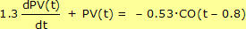
Aside: the FOPDT dynamic model has the general controller output (CO) to process variable (PV) form: 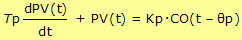
And this means we are claiming that the dynamic behavior of the heat exchanger can be reasonably approximated as: With units: t [=] min, PV(t) [=] °C, CO(t – Өp) [=] % The FOPDT model prediction for PV in the plot below was generated by solving the above differential equation using the actual CO signal trace as shown in the plot. |
The plot below (click for large view) compares step test data from the heat exchanger process to the FOPDT model using the parameters we computed in the previous articles.
Visual inspection reveals that the simple FOPDT model provides a very good approximation of the dynamic response behavior between the controller output (CO) signal and the measured process variable (PV) for this process.
This validates that, for the heat exchanger process at this design level of operation, we have good knowledge of:
| |
the direction the PV moves given a change in the CO |
| |
how far the PV ultimately travels for a given change in the CO |
| |
how fast the PV moves as it heads toward its new steady state |
| |
how much delay occurs between when the CO changes and the PV first begins to respond |
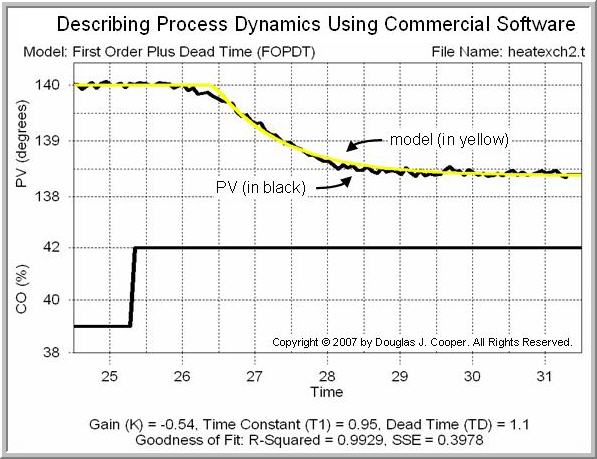
Modeling Using Software
For comparison, we show a FOPDT model fit (click for large view) of the same heat exchanger data using a software modeling tool (more discussion here). The model parameters are somewhat different and the model appears to match the PV data a little better based on a visual inspection.
We will leave it to later articles to discuss the benefits of commercial software for controller design and tuning. For now, it is enough to know that:
| |
the option is available, |
| |
FOPDT modeling can occur with just a few mouse clicks instead of using graph paper and hand calculations, and |
| |
the results are more descriptive when compared to the graphical method. |
With that said, graphical modeling is important to understand because it helps us isolate the role of each FOPDT model parameter, and in particular, appreciate what each says about the controller output (CO) to process variable (PV) relationship.
Using the Model in Controller Design
With a FOPDT model in hand, we can complete the controller design and tuning recipe to implement P-Only, PI, PID and PID with CO Filter control of the heat exchanger process.
The exciting result is that we achieve our desired controller performance using the information from this single step test. Our results are achieved quickly, there is no trial and error, we produce minimal off-spec product, and thus, there is no wasted time or expense.
The method of approximating complex behavior with a FOPDT model and then following a recipe for controller design and tuning has been proven on a wide variety of processes. In fact, it is an approach being used to improve profitability and safety in many plants today.