PI Control of the Heat Exchanger

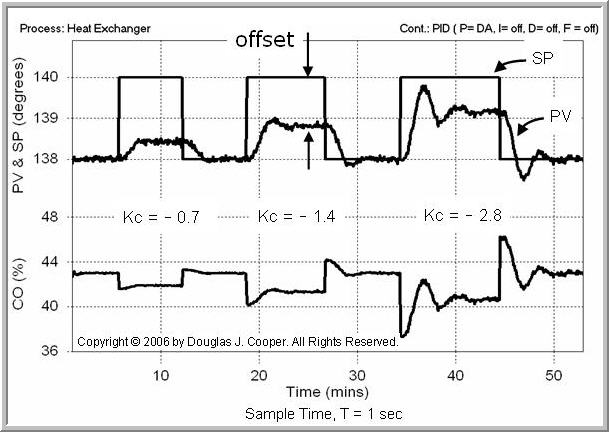
We investigated P-Only control of the heat exchanger process and learned that while P-Only is an algorithm that is easy to tune and maintain, it has a severe limitation. Specifically, its simple form permits steady state error, called offset, in most processes during normal operation.

Then we moved on to integral action and PI control. We focused in that article on the structure of the algorithm and explored the mathematics of how the proportional and integral terms worked together to eliminate offset.

Here we test the capabilities of the PI controller on the heat exchanger process. Our focus is on design, implementation and basic performance issues. Along the way we will highlight some strengths and weaknesses of this popular algorithm.

As with all controller implementations, best practice is to follow our proven four-stepdesign and tuning recipe as we proceed with this case study.

Step 1: Design Level of Operation (DLO)
Real processes display a nonlinear behavior. That is, their process gain, time constant and/or dead time changes as operating level changes and as major disturbances change. Since controller design and tuning is based on these process Kp, Tp and Өp values, controllers should be designed and tuned for a specific level of operation.

Thus, the first step in our controller design recipe is to specify our design level of operation (DLO). This includes stating:

We will track along with the same design conditions used in the P-Only control study to permit a direct comparison of performance and capability. As in that study, we specify:

▪ Design PV and SP = 138 °C with range of 138 to 140 °C

We also should know normal or typical values for our major disturbances and be reasonably confident that they are quiet so we may proceed with a bump test. The heat exchanger process has only one major disturbance variable, and consistent with the previous study:

▪ Expected warm liquid flow disturbance = 10 L/min

Step 2: Collect Data at the DLO
The next step in the design recipe is to collect dynamic process data as near as practical to our design level of operation. We have previously collected and documentedheat exchanger step test data that matches our design conditions.

Step 3: Fit an FOPDT Model to the Design Data
Here we document a first order plus dead time (FOPDT) model approximation of the step test data from step 2:
▪ Process gain (how far), Kp = –0.53 °C/%
▪ Time constant (how fast), Tp = 1.3 min
▪ Dead time (how much delay), Өp = 0.8 min

Step 4: Use the Parameters to Complete the Design
One common form of the PI controller computes a controller output (CO) action every loop sample time T as:

Where:
CO = controller output signal (the wire out)
CO_bias = controller bias or null value; set by bumpless transfer as explained below
e(t) = current controller error, defined as SP – PV
SP = set point
PV = measured process variable (the wire in)
Kc = controller gain, a tuning parameter
    Ti = reset time, a tuning parameter

• Loop Sample Time, T
  Best practice is to specify loop sample time, T, at 10 times per time constant or faster (T ≤ 0.1Tp). For this study, T ≤ 0.13 min = 8 sec. Faster sampling may provide modestly improved performance, while slower sampling can lead to significantly degraded performance.  Most commercial controllers offer an option of T = 1.0 sec, and since this meets our design rule, we use that here.
• Computing controller error, e(t)
  Set point, SP, is something we enter into the controller. The PV measurement comes from our sensor (our wire in). With SP and PV known, controller error, e(t) = SP – PV, can be directly computed at every loop sample time T.
• Determining Bias Value
  Strictly speaking, CO_bias is the value of the CO that, in manual mode, causes the PV to steady at the DLO while the major disturbances are quiet and at their normal or expected values.
• Bumpless Transfer
  A desirable feature of the PI algorithm is that it is able to eliminate the offset that can occur under P-Only control. The integral term of the PI controller provides this capability by providing updated information that, when combined with the controller bias, keeps the process centered as conditions change.

Since integral action acts to update (or reset) our bias value over time, CO_bias can be initialized in a straightforward fashion to a value that produces no abrupt control actions when we switch to automatic. Most commercial controllers do this with a simple “bumpless transfer” feature. When switching to automatic, they initialize:
▪ SP equal to the current PV
▪ CO_bias equal to the current CO

With the set point equal to the measured process variable, there is no error to drive a change in our controller output. And with the controller bias set to our current controller output, we are prepared by default to maintain current operation.

We will use a controller that employs these bumpless transfer rules when we switch to automatic. Hence, we need not specify any value for CO_bias as part of our design.

• Computing Controller Gain and Reset Time
  Here we use the industry-proven Internal Model Control (IMC) tuning correlations. The first step in using the IMC correlations is to compute Tc, the closed loop time constant. All time constants describe the speed or quickness of a response. The closed loop time constant describes the desired speed or quickness of a controller in responding to a set point change or rejecting a disturbance.

If we want an active or quickly responding controller and can tolerate some overshootand oscillation as the PV settles out, we want a small Tc (a short response time) and should choose aggressive tuning:
▪ aggressive:    Tc is the larger of 0.1·Tp  or  0.8·Өp

Moderate tuning is for a controller that will move the PV reasonably fast while producing little to no overshoot.
▪ moderate:     Tc is the larger of    1·Tp  or     8·Өp

If we seek a more sluggish controller that will move things in the proper direction, but quite slowly, we choose conservative tuning (a big or long Tc).
▪ conservative: Tc is the larger of  10·Tp  or   80·Өp

Once we have decided on our desired performance and computed the closed loop time constant, Tc, with the above rules, then the PI correlations for controller gain, Kc, and reset time, Ti, are:

Notice that reset time, Ti, is always set equal to the time constant of the process, regardless of desired controller activity.

1. a) Moderate Response Tuning:
   For a controller that will move the PV reasonably fast while producing little to no overshoot, choose:

Moderate Tc = the larger of 1·Tp or 8·Өp
= larger of 1(1.3 min) or 8(0.8 min)
= 6.4 min

Using this Tc and our model parameters in the tuning correlations above, we arrive at the moderate tuning values:

1. b) Aggressive Response Tuning:
   For an active or quickly responding controller where we can tolerate some overshoot and oscillation as the PV settles out, specify

Aggressive Tc = the larger of 0.1·Tp or 0.8·Өp
= larger of 0.1(1.3 min) or 0.8(0.8 min)
= 0.64 min

and the aggressive tuning values are:

• Controller Action
The process gain, Kp, is negative for the heat exchanger, indicating that when CO increases, the PV decreases in response. This behavior is characteristic of a reverse acting process. Given this CO to PV relationship, when in automatic mode (closed loop), if the PV starts drifting above set point, the controller must increase CO to correct the error. Such negative feedback is an essential component of stable controller design.

A process that is naturally reverse acting requires a controller that is direct acting to remain stable. In spite of the opposite labels (reverse acting process and direct acting controller), the details presented above show that both Kp and Kc are negative values.

In most commercial controllers, only positive Kc values can be entered. The sign (or action) of the controller is then assigned by specifying that the controller is either reverse acting or direct acting to indicate a positive or negative Kc, respectively.

If the wrong control action is entered, the controller will quickly drive the final control element (FCE) to full on/open or full off/closed and remain there until a proper control action entry is made.

Implement and Test
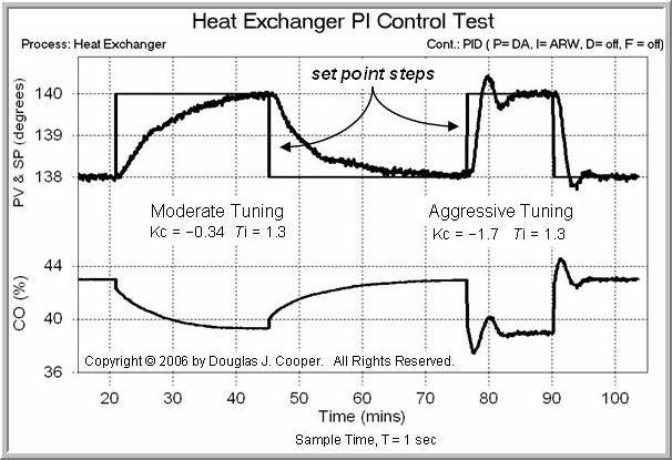
Below we test our two PI controllers on the heat exchanger process simulation (click for large view). Shown are two set points step pairs from 138 °C up to 140 °C and back again.

The first set point steps to the left show the PI controller performance using the moderate tuning values computed above. The second set point steps to the right show the controller performance using the aggressive tuning values. Note that the warm liquid disturbance flow, though not shown, remains constant at 10 L/min throughout the study.

(For comparison, the performance of the P-Only controller in tracking these set point changes is pictured here).

The asymmetrical behavior of the PV for the set point steps up compared to the steps down is due to the very nonlinear character of the heat exchanger.

If we seek tuning between moderate and aggressive performance, we would average the Kc values from the tuning rules above.

But if we believe we had collected good bump test data (we saw a clear response in the PV when we stepped the CO and the major disturbances were quiet during the test), and the FOPDT model fit appears to be visually descriptive of the data, then we have a good value for Tp and that means a good value for Ti.

If we are going to fiddle with the tuning, we can tweak Kc and we should leave the reset time alone.

Tuning Recipe Saves Time and Money
The exciting result is that we achieved our desired controller performance based on one bump test and following a controller design recipe. No trial and error was involved. Little off-spec product was produced. No time was wasted.

Soon we will see how software tools help us achieve such results with even less disruption to the process.

The method of approximating complex behavior with a FOPDT model and then following a recipe for controller design and tuning has been used successfully on a broad spectrum of processes with streams composed of gases, liquids, powders, slurries and melts. It is a reliable approach that has been proven time and again at diverse plants from a wide range of companies.