By Bob Rice1 and Doug Cooper
As has been discussed elsewhere in this e-book, it is best practice to follow a formal recipe when designing and tuning a PID controller. A recipe lets us move a controller into operation quickly. And perhaps most important, the performance of the controller will be superior to one tuned using an intuitive approach or trial-and-error method.
Additionally, a recipe-based approach overcomes many of the concerns that makes control projects challenging in an industrial operating environment. Specifically, a recipe approach causes less disruption to the production schedule, wastes less raw material and utilities, requires less personnel time, and generates less off-spec product.
The Recipe for Integrating Processes
Integrating (or non-self regulating) processes display counter-intuitive behaviors that make them surprisingly challenging to control. In particular, they do not naturally settle out to a steady operating level if left uncontrolled.
So while the controller design and tuning recipe is generally the same for both self regulating and integrating processes, there are important differences. Specifically, step 3 of the recipe uses a different dynamic model form and step 4 employs different tuning correlations.
Yet the design and tuning recipe maintains the familiar four step structure:
| 1. | Establish the design level of operation (the normal or expected values for set point and major disturbances). |
| 2. | Bump the process and collect controller output (CO) to process variable (PV) dynamic process data around this design level. |
| 3. | Approximate the process data behavior with a first order plus dead time integrating (FOPDT Integrating) dynamic model. |
| 4. | Use the model parameters from step 3 in rules and correlations to complete the controller design and tuning. |
It is important to recognize that real processes are more complex than the simple FOPDT Integrating model form used in step 3. In spite of this, the FOPDT Integrating model succeeds in providing an approximation of process behavior that is sufficiently accurate to yield reliable and predictable control performance when used with the rules and correlations in step 4 of the recipe.
The FOPDT Integrating Model
We recall that the familiar first order plus dead time (FOPDT) dynamic model used to approximate self regulating dynamic process behavior has the form:
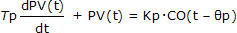 FOPDT Form
Yet this model cannot describe the kind of integrating process behavior shown in these examples. Such behavior is better described with the FOPDT Integrating model form:
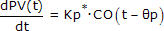 FOPDT Integrating Form
It is interesting to note when comparing the two models above that the FOPDT Integrating form does not have the lone “+ PV” term found on the left hand side of the FOPDT dynamic model.
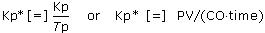
Also, individual values for the familiar process gain, Kp, and process time constant, Tp, are not separately identified for the FOPDT Integrating model. Instead, an integrator gain, Kp*, is defined that has units of the ratio of the process gain to the process time constant, or:
Tuning Correlations for Integrating Processes
Analogous to the FOPDT investigations on this site (e.g., here and here), we will see that the FOPDT Integrating model parameters Kp* and Өp of Step 3 can be computed using a graphical analysis of plot data or by automated analysis using commercial software.
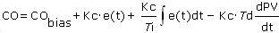
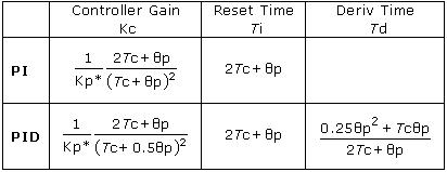
Step 4 then provides tuning values for controllers such as the dependent, ideal PI form:
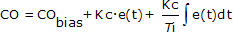
and the dependent, ideal PID form:
One important difference about integrating processes is that since there is no identifiable process time constant in the FOPDT Integrating model, we use dead time,Өp, as the baseline marker of time in the design and tuning rules.
Specifically, Өp is used as the basis for computing sample time, T, and the closed loop time constant, Tc. Following the procedures widely discussed on this site for self regulating processes (e.g. here and here), we employ a rule to compute the closed time constant, Tc, as:
Tc = 3Өp
The controller tuning correlations for integrating processes use this Tc, as well as the Kp* and Өp from the FOPDT integrating model fit, as:
Loop Sample Time, T
Determining a proper sample time, T, for integrating processes is somewhat more challenging than for self regulating processes.
As discussed in this article, there are two sample times, T, used in process controller design and tuning. One is the control loop sample time that specifies how often the controller samples the measured process variable (PV) and computes and transmits a new controller output (CO) signal. The other is the rate at which CO and PV data are sampled and recorded during a bump test (step 2 of the recipe).
Also discussed in that article is that all controllers measure, act, then wait until next sample time before repeating the loop. This “measure, act, wait” procedure has a delay (or dead time) of one sample time built naturally into its structure. Thus, the minimum dead time (Өp,min) in any control loop is the loop sample time, T.
With this information, we recognize a somewhat circular argument in defining sample time for integrating processes:
 our time basis for controller design is Өp, and as such, then loop sample time, T, should be small relative to dead time, or:
T ≤ 0.1Өp
but the minimum that dead time can be is one sample time, T, or
Өp,min = T
Thus, T is based on Өp, and if the process is sampled too slowly during a bump test, then Өp can be based on T.
To avoid this issue, it is best practice to sample the process as fast as reasonably possible during bump tests so accurate model parameters can be determined during analysis. Loop sample time, T, can then be computed from dead time for controller implementation.
If there is concern about a particular analysis, an alternative and generally conservative way to compute sample time is:
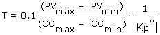
where the subscripts max and min refer to the maximum and minimum values for CO and PV across the signal span of the instrumentation.
Using the Recipe
The tuning recipe for integrating processes has important differences from that used for self regulating process. When designing and tuning controllers for such processes, we should:
use an FOPDT Integrating model form when approximating dynamic model behavior,
note that the closed loop time constant, Tc, and sample time, T, are based on model dead time, Өp.
employ PI and PID tuning correlations specific to integrating processes.
_______
1. Bob Rice holds primary responsibility at Control Station for training and software development, deployment, and support. Dr. Rice has published extensively on topics associated with automatic process control, including non-self-regulating processes and model predictive control. Prior to joining Control Station, Dr. Rice held engineering and technical positions with PPG Industries and The Walt Disney Company.
Robert Rice, Ph.D.
Director of Solutions Engineering
Control Station, Inc.
One Technology Drive
Tolland, CT 06084
Phone: (860) 872-2920
Email: bob.rice@controlstation.com
Web: http://www.controlstation.com/