When improved disturbance rejection performance is our goal, one benefit of a cascade control (nested loops) architecture over a feed forward strategy is that implementing a cascade builds upon our existing skills.
The cascade block diagram is presented in the graphic below (click for a large view) and discussed in detail in this article. As shown, a cascade has two controllers. Implementation is a familiar task because the procedure is essentially to employ ourcontroller design and tuning recipe twice in sequence.
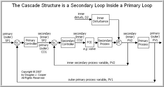
The cascade architecture variables listed in the block diagram include:
CO2 = inner secondary controller output signal to the FCE
PV2 = the early warning inner secondary process variable
SP2 = CO1 = inner secondary set point equals the outer primary controller output
PV1 = outer primary process variable
SP1 = outer primary set point
D2 = disturbances that impact the early warning PV2 before they impact PV1
FCE = final control element (e.g., a valve) is continuously adjustable between on/open and off/closed, and that impacts PV2 before it impacts PV1
Two Bump Tests Required
Two bump tests are required to generate the dynamic process response data needed to design and tune the two controllers in a cascade implementation.
• First the Inner Secondary Controller
A reliable procedure begins with the outer primary controller in manual mode (open loop) as we apply the design and tuning recipe to the inner secondary controller.
Thus, with our process steady at (or as near as practical to) its design level of operation (DLO), we generate dynamic CO2 to PV2 process response data with either amanual mode (open loop) bump test or a more sophisticated SP driven (closed loop)bump test.
The objective for the inner secondary controller is timely rejection of disturbances D2 based on the measurement of an “early warning” secondary process variable PV2. Good disturbance rejection performance is therefore of fundamental importance for the inner secondary controller.
Yet as shown in the block diagram above and detailed in this article, the output signal of the outer primary controller becomes a continually updated set point for the inner secondary controller (SP2 = CO1). Since we expect the inner secondary controller to respond crisply to these rapidly changing set point commands, it must also be tuned to provide good SP tracking performance.
In the perfect world, we would balance disturbance rejection and set point tracking capability for the inner secondary controller. But we cannot shift our attention to the outer primary controller until we have tested and approved the inner secondary controller performance.
In production processes with streams comprised of gases, liquids, powders, slurries and melts, disturbances are often unmeasured and beyond our ability to manipulate at will. So while we desire to balance disturbance rejection and set point tracking performance for the inner secondary controller, in practice, SP tracking tests tend to provide the most direct route to validating inner secondary controller performance.
• Then the Outer Primary Controller
Once implemented, the inner secondary controller literally becomes part of the “process” from the outer primary controller’s view.
As a result, any alteration to the inner secondary controller (e.g., tuning parameter adjustments, algorithm modifications, sample time changes) can change the process gain, Kp, time constant, Tp, and/or dead time, Өp, of the outer loop CO1 to PV1 dynamic response behavior. This, in turn, impacts the design and tuning of the outer primary controller.
Thus, we must design, tune, test, accept and then “lock down” the inner secondary controller, leaving it in automatic mode with a fixed configuration. Only then, with our process steady and at (or very near) its DLO, can we proceed with the second bump test to complete the design and tuning of the outer primary controller.
Software Provides Benefit
Given that the outer primary controller design and tuning is based on the specifics of the inner secondary loop, a guess and test approach to a cascaded implementation can prove remarkably wasteful, time consuming and expensive.
In production operations, a commercial software package that automates the controller design and tuning tasks will pay for itself as early as a first cascade tuning project
Minimum Criteria for Success
A successful cascade implementation requires that early warning process variable PV2 respond before outer primary PV1 both to disturbances of concern (D2) and to final control element (FCE) manipulations (e.g., a valve).
Responding first to disturbances means that the inner secondary D2 to PV2 dead time,Өp, must be smaller than the overall D2 to PV1 dead time, or:
Өp (D2 −› PV2) < Өp (D2 −› PV1)
Responding first to FCE manipulations means that the inner secondary CO2 to PV2 dead time must be smaller than the overall CO2 to PV1 dead time, or:
Өp (CO2 −› PV2) < Өp (CO2 −› PV1)
If these minimum criteria are met, then a cascade control architecture can show benefit in improving disturbance rejection.
P-Only vs. PI for Inner Secondary Controller
A subtle design issue relates to the choice of control algorithm for the inner secondary controller. While perhaps not intuitive, an inner secondary P-Only controller will provide better performance than a PI controller in many cascade implementations.
• Defining Performance
We focus all assessment of control performance on outer primary process variable PV1. Performance is “improved” if the cascade structure can more quickly and efficiently minimize the impact of disturbances D2 on PV1. Given the nature of the cascade structure, it is assumed that D2 first disrupts PV2 as it travels to PV1.
Since PV2 was selected because of its value as an early warning variable, our interest in PV2 control performance extends only to its ability to provide protection to outer primary process variable PV1. We are otherwise unconcerned if PV2 displays offset, shows a large response overshoot, or any other performance characteristic that might be considered undesirable in a traditional measured PV.
• Is the Inner Loop “Fast” Relative to the Overall Process?
A cascade architecture with a P-Only controller on the inner secondary loop will provide improved disturbance rejection performance over that achievable with a traditional single loop controller if the minimum criteria for success as discussed above are met.
A PI controller on the inner loop may provide even better performance than P-Only, but only if the dynamic character of the inner secondary loop is “fast” relative to that of the overall process.
If the inner secondary loop dynamic character is not sufficiently fast, then a PI controller on the inner loop, even if properly designed and tuned, will not perform as well as P-Only. It is even possible that a PI controller could degrade performance to an extent that the cascade architecture performs worse than a traditional (non-cascade) single loop controller.
• Why PI controllers Need a “Fast” Inner Loop
At every sample time T, the outer primary controller computes a controller output signal that is fed as a new set point to the inner secondary controller (CO1 = SP2). The inner secondary controller continually makes CO2 moves as it works to keep PV2 equal to the ever-changing SP2.
The cascade will fail if the inner loop cannot keep pace with the rapid-fire stream of SP2 commands. If the inner secondary controller “falls behind” (or more specifically, if the CO2 actions induce dynamics in the inner loop that do not settle quickly relative to the dynamic behavior of the overall process), the benefit of the early warning PV2 measurement is lost.
A P-Only controller can provide energetic control action when tracking set points and rejecting disturbances. Its very simplicity can be a useful attribute in a cascade implementation because a P-Only controller quickly completes its response actions to any control error (E2 = SP2 – PV2). While P-Only controllers display offset when operation moves from the DLO, this is not considered a performance problem for inner secondary PV2.
With two tuning parameters, a PI controller has a greater ability to track set points and reject disturbances. However, this added sophistication yields a controller with a greater tendency to “roll” or oscillate. And the ability to eliminate offset, normally considered a positive attribute for PI controllers, can require a longer series of control actions that extends how quickly a loop settles.
Thus, a PI controller generally needs more time (a faster inner loop) to exploit its enhanced capability relative to that of a P-Only controller. If the dynamic nature of a particular cascade does not provide this time, then an inner-loop P-Only controller is the proper choice.
The Cascade Implementation Recipe
Below is a generally conservative approach for cascade control implementation. Note that the recipe assumes that:
| ▪ | Early warning PV2 responds before PV1 both to D2 and CO2 changes as discussed above in the minimum criteria for cascade success. |
| ▪ | A first order plus dead time (FOPDT) model of dynamic process data yields a process time constant, Tp, that is much larger than the dead time, Өp. This permits us to focus on the time constant as the marker for “fast” dynamic process behavior. |
1) Starting from a steady operation, step, pulse or otherwise perturb CO2 around the design level of operation (DLO). Collect CO2, PV2 and PV1 dynamic data as the process variables respond. The inner secondary loop can be in automatic (closed loop) if the controller is sufficiently active to force a clear dynamic response in PV2. The outer primary loop is normally in manual (open loop).
2) Fit a FOPDT model to the inner secondary process (CO2 −› PV2) data and another to the overall process (CO2 −› PV1) data, yielding:
| Inner Secondary | Overall Process | |
| Process Gain (how far) | Kp (CO2 −› PV2) | Kp (CO2 −› PV1) |
| Time Constant (how fast) | Tp (CO2 −› PV2) | Tp (CO2 −› PV1) |
| Dead Time (how much delay) | Өp (CO2 −› PV2) | Өp (CO2 −› PV1) |
Note from the block diagram at the top of the article that the inner secondary process dynamics are contained within the overall process dynamics. Therefore, the physics of a cascade implies that the time constant and dead time values for the inner process will not be greater than those of the overall process, or:
Tp (CO2 −› PV2) ≤ Tp (CO2 −› PV1) and Өp (CO2 −› PV2) ≤ Өp (CO2 −› PV1)
3) Use the time constants to decide whether the inner secondary dynamics are fast enough for a PI controller on the inner loop.
Case 1: If the inner secondary process is not at least 3 times faster than the overall process, it is not fast enough for a PI controller.
• If 3×Tp (CO2 −› PV2) > Tp (CO2 −› PV1) => Use P-Only controllerCase 2: If the inner process is 3 to 5 times faster than the overall process, then P-Only will perform similar to PI control. Use our own preference.
• If 3×Tp (CO2 −› PV2) ≤ Tp (CO2 −› PV1) ≤ 5×Tp (CO2 −› PV2) => Use either P-Only or PI controllerCase 3: If the inner process is more than 5 times faster than the overall process, it is “fast” and a PI controller will provide improved performance.
• If 5×Tp (CO2 −› PV2) < Tp (CO2 −› PV1) => Use PI controller
4) When we have determine whether the inner secondary controller should be a P-Only or PI algorithm, we tune it and test it. Once acceptable performance has been achieved, leave the inner secondary controller in automatic; it now literally becomes part of the outer primary process.
5) Select an algorithm with integral action for the outer primary controller (PI, PID orPID with CO filter) to ensure that offset is eliminated. Tune the primary controller using the design and tuning recipe. Note that bumping the outer primary process requires stepping, pulse or otherwise perturbing the set point (SP2) of the inner secondary controller.
6) With both controllers in automatic, tuning of the cascade is complete.
Cascade Control of the Jacketed Stirred Reactor
Once a cascade control architecture is put in service, we must remember that every time the inner secondary controller is changed in any way, the outer primary controller should be reevaluated for performance and retuned as necessary.
We should also be aware that the recipe presented above is a general procedure intended for broad application. Thus, there will be occasional exceptions to the rules.
We next explore a case study on the cascade control of the jacketed stirred reactor.