Ziegler and Nichols first proposed their method in 1942. It is a trial-and-error loop tuning technique that is still widely used today. The automatic mode (closed-loop) procedure is as follows:
| ▪ | Set our controller to P-Only action and switch it to automatic when the process is at the design level of operation. |
| ▪ | Guess an initial controller gain, Kc, that we expect (hope) is conservative enough to keep the loop stable. |
| ▪ | Bump the set point a small amount and observe the response behavior. |
| ▪ | If the controller is not causing the measured process variable (PV) to sustain an oscillating pattern, increase the Kc (or decrease the proportional band, PB) and wait for the new response. |
| ▪ | Keep adjusting and observing by trail and error until we discover the value of Kc that causes sustained uniform oscillations in the PV. These oscillations should neither be growing nor dying out, and the controller output (CO) should remain unconstrained. |
| ▪ | The controller gain at this condition is called the ultimate gain, Ku. The period of the PV oscillation pattern at the ultimate gain is called the ultimate period, Pu. |
After using the procedure above to determine the ultimate gain and ultimate period, the Ziegler-Nichols (Z-N) correlations to compute our final tuning for a PI controller are:
• Ziegler-Nichols PI Tuning: Kc = 0.45∙Ku Ti = Pu/1.2
Many process control books and articles propose a variety of tuning correlations using Ku and Pu that provide improved performance over that provided by the original Z-N correlations listed above. Of course, the definition of “improved” can vary widely depending on the process being controlled and the operations staff responsible for a safe and profitable operation.
Ziegler-Nichols Applied to the Heat Exchanger
To illustrate the procedure, we apply it to the same heat exchanger process explored in numerous articles in this e-book.
Below is a plot (click for a large view) showing the heat exchanger under P-Only control. The controller gain, Kc, is initially set to Kc = –1.0 %/°C, a value we hope provides conservative performance as we start our guess and test investigation.
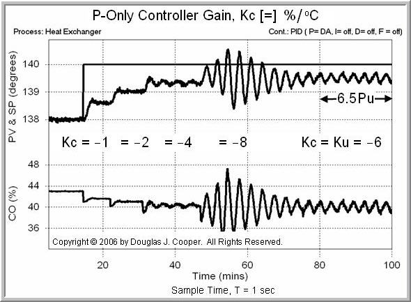
As shown above, the process is perturbed with a set point step and we wait to see if the controller yields sustained oscillations. The process variable (PV) displays a sluggish response at Kc = –1.0 %/°C, so we double the controller gain to Kc = –2.0 %/°C, and then double it again to Kc = –4.0 %/°C, waiting each time for the response pattern to establish itself.
When changing from a Kc = –4.0 up to Kc = –8.0 %/°C as shown in the above plot at about time t = 45 min, the heat exchanger goes unstable as evidenced by the rapidly growing oscillations in the PV. This indicates we have gone too far and must back down on the P-Only controller gain.
A compromise of Kc = –6.0 %/°C seems to create our desired goal of a process teetering on the brink of stability. Hence, we record our ultimate gain as:
Ku = –6 %/°C
As indicated in the plot above from time t = 80 min through t = 100 min, when under P-Only control at our ultimate gain, the PV experiences 6.5 complete cycles or periods of oscillation over 20 minutes. The ultimate period, Pu, is thus computed as:
Pu = 20 min/6.5 = 3.1 min
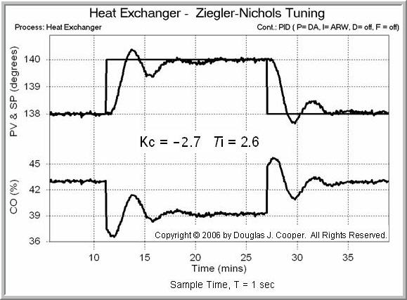
We employ these Ku and Pu values in the Z-N correlations above to obtain our PI tuning values:
• Kc = 0.45∙Ku = 0.45 (–6 %/°C) = –2.7 %/°C
• Ti = Pu/1.2 = 3.1 min/1.2 = 2.6 min
Below (click for a large view) is the performance of this Z-N tuned PI controller in tracking a set point step from 138 °C up to 140 °C. For comparison, the heat exchanger responding to the same set point steps using an IMC tuned PI controller is shown here.
Concerns in a Production Environment
Suppose we were using the Z-N closed-loop method to tune the above controller in a production environment:
1) The trial and error search for the ultimate gain took about 80 minutes in the test above. For comparison, consider that the single step test for the IMC design on the heat exchanger took only 5 minutes.
Even if there is suspicion that we skewed the process testing to make Z-N look bad, the fact remains that it will always take significantly longer to find the ultimate gain by trial and error then it will to perform a simple bump test.
And in a production situation, this means we are losing time and wasting money as we make bad product. Why even consider such a time-consuming and wasteful tuning method when it is not necessary?
2) Perhaps more significant, the Z-N method requires that we literally bring our process to the brink of instability as we search for the ultimate gain. Creeping up on the ultimate gain can be very time consuming (and hence very expensive), but if we try to save time by making large adjustments in our search for Ku, it becomes much more likely that we will actually go unstable, at least for a brief period.
In production situations, especially involving reactors, separators, furnaces, columns and such, approaching an unstable operation is an alarming proposition for plant personnel.
Final thoughts
This e-book focuses on the control of processes with streams composed of liquids, gases, powders, slurries and melts. The challenging control problems for such process are most always found in a production environment.
Our controller design and tuning recipe is designed specifically for such situations. It’s fast and efficient, saves time and money, and provides consistent and predictable performance.