There are two sample times, T, used in process controller design and tuning.
One is the control loop sample time (step 4 of the design and tuning recipe) that specifies how often the controller samples the measured process variable (PV) and computes and transmits a new controller output (CO) signal.
The other is the rate at which CO and PV data are sampled and recorded during a bump test (step 2 of the recipe).
In both cases, sampling too slow will have a negative impact on performance. Sampling fast will not necessarily provide better performance, though it may lead us to spend more than necessary on high-end instrumentation and computing resources.
Fast and slow are relative terms defined by the process time constant, Tp. Best practice for both control loop sample time and bump test data collection are the same:
| Best Practice: Sample time should be 10 times per process time constant or faster (T ≤ 0.1Tp). |
In this article we explore both sample time issues. Specifically, we study:
| 1) | The impact on performance when we adjust control loop sample time while keeping the tuning of a PI controller fixed, and |
| 2) | How performance is affected when we sample a process at different rates during a bump test and then complete the controller design and tuning using this same T. |
The Process
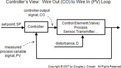
Like all articles on this site, the CO and PV data we consider are the wire out to wire insamples collected at the controller interface. Thus, as shown below, the equipment (e.g., actuator, valve, process unit, sensor, transmitter) and analog or digital manipulations (e.g., scaling, filtering, linearization) are all lumped as a single “process” that sits between the CO and PV values.
To provide the ability to manipulate and monitor all aspects of an orderly investigation, we use a differential equation (or transfer function) simulation utility to create the overall process.
It is not necessary to understand the simulation utility to appreciate and learn from the studies below. But for those interested, we provide a screen grab (click for large view) from the commercial software used for this purpose:
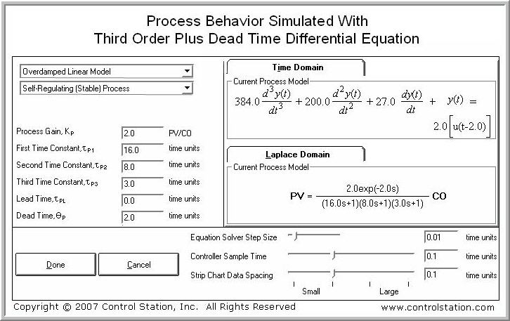
This same “process” is used in all examples in this article. Though expressed as a linear equation, it is sufficiently complex that the observations we make will be true for a broad range of process applications.
The Disturbance
Real processes have many disturbances that can disrupt operation and require corrective action from the controller. For the purposes of this investigation, we focus on only one generic disturbance (D) to our process.
The manner in which a PV responds to a disturbance is different for every application. Given this, here we choose a middle ground. Specifically, we specify that the impact of D on PV is exactly the same as the impact of CO on PV.
Thus, the D to PV behavior is simulated in the examples with the identical differential equation as shown above for the CO to PV behavior. This assumption is not right or wrong or good or bad. In fact, it is a rather common assumption in theoretical studies. Our goal is simply to provide a basis of comparison when we start exploring how sample time impacts controller performance.
The PI Controller
All examples in this article use the PI controller form:
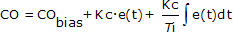
where algorithm parameters are defined here.
The PI controller computes a CO action every loop sample time, T. To best highlight differences based on sample time issues, we choose an aggressive controller tuning as detailed in this example. Tuning parameters are thus computed based on an approximating first order plus dead time (FOPDT) model fit (step 3 of the recipe) as:
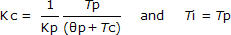 where: Tc is the larger of 0.1·Tp or 0.8·Өp
Parameter Units
Time is expressed as generic “time units” and is not listed in the plots, calculations or tables. The conclusions we draw are independent of whether these are milliseconds, seconds, minutes or any other time units.
It is important to recognize, however, that when applying the observations from this article to other applications, we must be sure that all time-related parameters, including sample time, dead time, time constants and reset time, are expressed in consistent units. They should all be in seconds or all be in minutes, for example.
CO and PV both range from 0-100% in the examples. Process gain, Kp, thus has units of (% of PV)/(% of CO), while controller gain, Kc, units are (% of CO)/(% of PV).
For the remainder of this article, all parameters follow the above units convention. While something we normally avoid as bad practice, units are not explicitly displayed in the various plots and calculations.
(1) Impact of Loop Sample Time When Controller Tuning is Constant
In this first study, we follow the recipe to design and tune a PI controller for the process above. Set point tracking performance is then explored as a function of control loop sample time, T.
• Step 1: Establish the Design Level of Operation (DLO)
We arbitrarily initialize CO, PV, SP and D all at 50% and choose this as the default DLO.
• Step 2: Collect CO to PV bump test data around the DLO
The plot in step 3 shows the bump test data used in this study. The sample time used during data collection is T = 0.1, which we confirm in step 3 is a very fast T = 0.005Tp.
• Step 3: Approximate the Process Behavior with an FOPDT Dynamic Model
We use commercial software to fit a first order plus dead time (FOPDT) model to the dynamic process data as shown below (click for large view). This fit could also be performed by hand using a graphical analysis of the plot data following the methodsdetailed here.
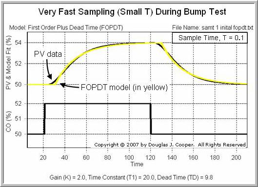
The FOPDT model fit (in yellow) visually matches the PV data in the plot, so we accept the model as an appropriate approximation of the more complex dynamic process behavior. The model parameters are listed beneath the plot and are summarized here:
▪ Process gain (how far), Kp = 2.0
▪ Time constant (how fast), Tp = 20
▪ Dead time (how much delay), Өp = 9.8
• Step 4: Use the FOPDT Model Parameters to Complete the Design and Tuning
Using the Kp, Tp and Өp from step 3, we first compute the closed loop time constant,Tc, for an aggressively tuned controller as:
Aggressive Tc = the larger of 0.1·Tp or 0.8·Өp
= larger of 0.1(20) or 0.8(9.8)
= 7.8
and then using the tuning correlations listed earlier, we compute PI tuning values:
We implement these Kc and Ti values and hold them constant for the next three plots as we adjust control loop sample time, T.
The “best practice” design rule at the top of this article states that sample time should be 10 times per process time constant or faster (T ≤ 0.1Tp). Hence, the maximum sample time we should consider is: Tmax= 0.1Tp = 0.1(20) = 2.0
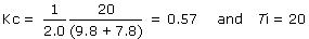
The plot below (click for large view) shows the set point tracking performance of the PI controller with fixed tuning when the sample time T is very fast (T = 0.1), fast (T = 0.5)and right at the maximum best practice value (T = 2.0).
The plot above supports that a control loop sample time smaller (faster) than the “maximum best practice” 0.1Tp rule has modest impact on performance.
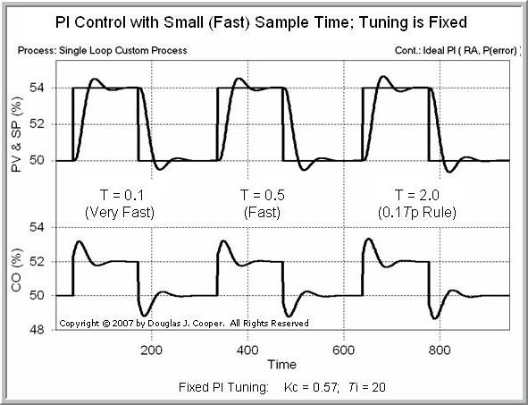
In the plot below (click for large view), we increase control loop sample time above the best practice limit. Because the scaling on the plot axes has changed from that above, we begin with the maximum best practice value of T = 0.1Tp = 2.0, and then test performance when the loop sample time is slow (T = 10) and very slow (T = 20) relative to the rule.
Performance of a controller with fixed tuning clearly degrades as loop sample time, T, increases above the maximum best practice value of 0.1Tp.
To better understand why, we zoom in on the control performance when loop sample time is very slow (T = 20). The plot below (click for large view) is a close-up from the plot above.
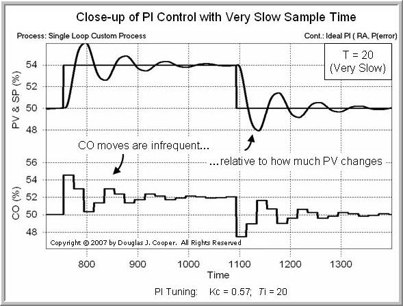
In the “very slow sample time” plot above, T = Tp. That is, the controller measures and acts only once per process time constant.
We can see in the plot that PV moves a considerable amount between each corrective CO action. At this slow sample time, the controller simply cannot keep up with the action and the result is a degraded control performance.
(2) Impact of Data Collection Sample Time During Bump Test
In this study we sample our process at different rates, T, during a bump test, complete the design and tuning, and then test the performance of the resulting controller using this same T as the control loop sample time. Following our recipe:
• Step 1: Establish the Design Level of Operation (DLO)
We again initialize CO, PV, SP and D all at 50% and choose this as the default DLO.
• Step 2: Collect CO to PV bump test data around the DLO
The plots in step 3 show identical bump tests. The only difference is the sample time used to collect and record data as the PV responds to the CO steps. We consider three cases:
▪ sample 10 times faster than rule: T = 0.01Tp = 0.2
▪ sample at the maximum “best practice” rule: T = 0.1Tp = 2
▪ sample 10 times slower than rule: T = Tp = 20
• Step 3: Approximate the Process Behavior with an FOPDT Dynamic Model
We again use Control Station software to fit a first order plus dead time model to each response plot (for a large view of the plots below, click T = 0.2; T = 2; T = 20)
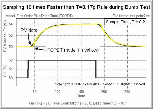

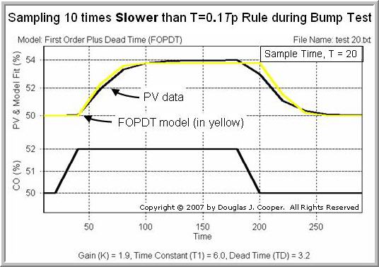
As the above plots reveal, an FOPDT model of the same process can be different if we sample and record data at different rates during a bump test.
Our best practice rule is based on the process time constant (Tp), a value we may not even know until after we have conducted our data collection experiment. If we do not know what to expect from a process based on prior experience, we recommend a “faster is better” attitude when sampling and recording data during a bump test.
• Step 4: Use the FOPDT Model Parameters to Complete the Design and Tuning
We summarize the Kp, Tp and Өp for the three cases in the table below. The first two columns (“sample fast” and “T = 0.1Tp rule”) show similar values. The “sample slow” column contains values that are clearly different.
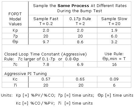
The tuning values shown in the bottom two rows across the table are computed by substituting the FOPDT model values into the PI tuning correlations as discussed earlier in this article.
The “Өp,min = T” rule for controller tuning
We do confront one new tuning issue in this study that merits discussion.
Consider that all controllers measure, act, then wait until next sample time; measure, act, then wait until next sample time. This “measure, act, wait” procedure has a delay (or dead time) of one sample time built naturally into its structure.
By definition, the minimum dead time, Өp, in a control loop is the loop sample time, T. Dead time can certainly be larger than T (and it usually is), but it cannot be smaller.
Thus, whether by software or graphical analysis, if we compute a Өp that is less than T, we must set Өp = T everywhere in our tuning correlations. This is the “Өp,min = T” rule for controller tuning.
In the “sample slow” case, we know that we will be using T = 20 when we implement the controller. So even though the FOPDT model fit yields a Өp = 3.2, we use Өp = 20 when computing both Tc and Kc as listed in the table.
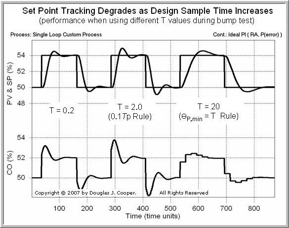
The plot below (click for large view) shows the set point tracking performance of three controllers, each designed and then implemented using three different sample times.
Below (click for large view) we show the performance of the three PI controllers in rejecting a disturbance. As discussed earlier in this article, recall that the D to PV dynamics are assumed to be identical to those of the CO to PV behavior.
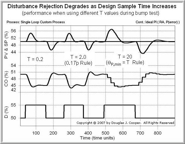
We should note that if we were to use Өp = 3.2 when computing tuning values for the “sample slow” case, the controller would be wildly unstable. Even with the Өp,min = T rule, performance is noticeably degraded compared to the other cases.
Final Thoughts
1) The “best practice” rule that sample time should be 10 times per process time constant or faster (T ≤ 0.1Tp) provides a powerful guideline for setting an upper limit on both control loop sample time and bump test data collection sample time.
2) Sampling as slow as once per Tp during data collection and then controller implementation can produce a stable, though clearly degraded, controller. Be sure to follow the “Өp,min = T” rule when using the controller tuning correlations to achieve a stable result.