We have investigated a graphical analysis method for fitting a first order plus dead time (FOPDT) dynamic model to step test data for both the heat exchanger and the gravity drained tanks processes in previous articles.
Describing process behavior with an approximating FOPDT dynamic model is the third step of our controller design and tuning recipe. Thus, it is a critical step for quickly achieving desired controller performance while avoiding time consuming and expensive trial and error methods.
The reason we studied graphical modeling is because it is a useful way to isolate the role of each FOPDT model parameter, and in particular, appreciate what each says about a controller output (CO) to process variable (PV) relationship.
As we learned in these investigations, for a change in CO:
▪ Process gain, Kp, describes the direction and how far the PV moves,
▪ Time constant, Tp, describes how fast the PV responds,
▪ Dead time, Өp, describes how much delay occurs before the PV first begins to move.
But in industrial practice, graphical modeling methods are very limiting for (at least) two reasons.
First, they restrict us to often-impractical step test data. With software, we can fit models to a broad range of dynamic data sets, including closed loop (automatic mode)set point response data.
And instead of using pencil, paper, calculator and ruler to analyze a step test, software can produce a reliable fit and present the results for our inspection almost as fast as we can click on the program icons.
Software Requires Electronic Data
One requirement for using a commercial software package for dynamic modeling and controller design is that the process data must be available in some sort of electronic form, ranging from a simple text file to an Excel spreadsheet format.
If the controller for the loop being modeled is software based (such as on a DCS), if the hardware is OPC enabled, if the controller is connected to a data historian, or if we have capable in-house tech support, then we should have access to process data in a file format.
| Practitioner’s note: If you believe process control is important to plant safety and profitability, yet your process data is not available in an electronic format, then perhaps your management is not convinced that process control is important to plant safety and profitability. |
The file must contain the sampled CO signal paired with the corresponding PV measurement for the entire bump test. If the data was collected at a constant sample rate, T, then we also must know this value. Otherwise, the data file must match each CO and PV pair with a sample time stamp.
Model Fitting of Doublet Data
For our gravity drained tanks study, we have previously discussed that the PV is liquid level in the lower tank, that the set point, SP, is held constant during production, and that our main objective is rejecting disruptions from D, the pumped flow disturbance.
We also presented process data from a doublet test around our design level of operation (DLO), which for this study is:
▪ design PV and SP = 2.2 m with range of 2.0 to 2.4 m
▪ design D = 2 L/min with occasional spikes up to 5 L/min
A doublet test, as shown below, is two CO pulses performed in rapid succession and in opposite direction. The second pulse is implemented as soon as the process has shown a response to the first pulse that clearly dominates the noise in the PV. It is not necessary to wait for the process to respond to steady state for either pulse.
The doublet test offers important benefits as a testing method, including that it starts from and quickly returns to the DLO. It also produces data both above and below the design level to “average out” the nonlinear effects. And the PV always stays close to the design level of operation, thus minimizing off-spec production.
Using the commercial software offered by Control Station, Inc, we read our data file into the software, select “First Order Plus Dead Time” from the model library, and then click “fit model.”
The results of the automated model fit are displayed below (click for a large view):

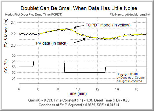
The sampled data is the black trace in the above plot and the FOPDT model is displayed in yellow. The model parameters from the doublet test model fit (shown below the plot) are listed in the table below.
For comparison, the results from our previous step analysis are also listed:

The software model fit is consistent with the step test graphical analysis. The extra accuracy of the computer output, though displayed by the software, does not necessarily hold significance as process data rarely contains such precise dynamic information. For real processes, these numbers are essentially equal.
Model Fit Minimizes SSE
The model fitting software performs a systematic search for a combination of model parameters that minimizes the sum of squared errors (SSE), computed as:
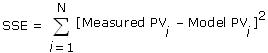
The Measured PV is the actual data collected from our process. The Model PV is computed using the model parameters from the search routine and the actual CO data from the file. N is the total number of samples in the file.
In general, the smaller the SSE, the better the model describes the data.
Software Offers Benefits
When the external disturbances and noise in the PV signal are small, the doublet can be quite modest in size yet still yield data for a meaningful fit as shown below (click for a large view):
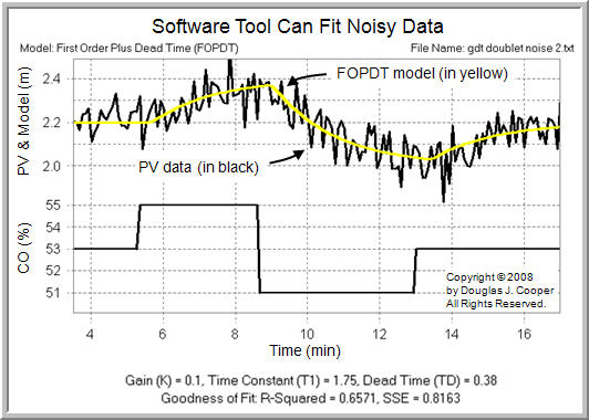
As shown below (click for a large view), software can also model data that contains significant noise in the PV signal, as long as the external disturbances are quiet.
For comparison, the model parameters from all of the above fits are summarized below:
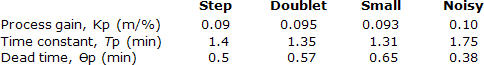
From a controller design and tuning perspective, each set of model parameters are similar enough that each will yield a controller with virtually identical performance and capability.
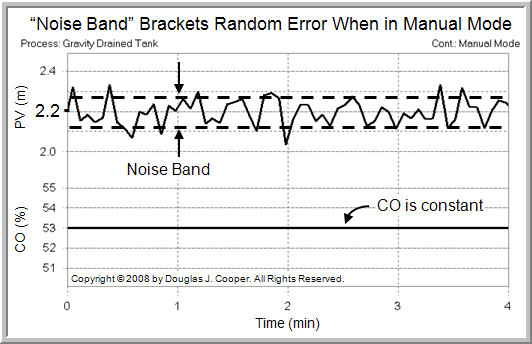
Noise Band Guides Test
When generating dynamic process data, it is important that the CO change is large enough and fast enough to force a response in the measured PV that clearly dominates the higher-frequency signal noise and lower-frequency random process variations.
One way to quantify the amount of noise and random variation for a process is with a noise band.
While there are formal approaches to defining a noise band, a simple approach as illustrated below (click for a large view) is to:
| ▪ | collect data for a period of time when the CO is held constant (i.e. the controller is in manual). |
| ▪ | draw lines that bracket most of the data. |
| ▪ | the separation in the brackets is the “noise band.” |
If the data is to be used for modeling, it is best practice to make changes in the CO that force the PV to move at least 5 times the noise band. In fact, some experts recommend that the PV moves 10 times the noise band to ensure a reliable result.
The noisy doublet example above did not meet this noise band rule, yet the fit was still reasonable. This is true in part because the process is a simulation and we could be certain that no process disturbances occurred to corrupt the data.
Advances in software also enable us to extract more information from a data set, which is why the noise band rule mentioned above has grown smaller in recent years.
Step 4: Controller Tuning and Testing
In later articles, we use the above model data and move quickly through the range of PID controllers. We focus on disturbance rejection and highlight the differences and similarities with the set point tracking studies we presented for the heat exchanger process.