Our control objective for the jacketed stirred reactor is to maintain reactor exit stream temperature at set point in spite of disturbances caused by a changing cooling liquid temperature entering the vessel jacket. In previous articles, we have established thedesign level of operation for the reactor and explored the performance of a single loop PI controller and a PID with CO Filter controller in meeting our control objective.
We also have proposed a cascade control architecture for the reactor that offers potential for improving disturbance rejection performance. We now apply our proposed architecture following the implementation recipe for cascade control. Our goal is to demonstrate the implementation procedure, understand the benefits and drawbacks of the method, and explore cascade disturbance rejection performance for this process.
The Reactor Cascade Control Architecture
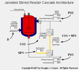
The reactor cascade architecture has been detailed in a previous article and is shown in the graphic below (click for a large view):
where:
CO2 = controller output to valve that adjusts cooling jacket liquid flow rate (%)
PV2 = cooling jacket outlet temperature is our “early warning” process variable (oC)
SP2 = CO1 = desired cooling jacket outlet temperature (oC)
PV1 = reactor exit stream temperature (oC)
SP1 = desired reactor exit stream temperature (oC)
D = temperature of cooling liquid entering the jacket (oC)
Design Level of Operation (DLO)
The details and discussion for our DLO are presented in this article and are summarized:
▪ Design PV1 and SP1 = 90 oC with approval for brief dynamic testing of ±2 oC
▪ Design D = 43 oC with occasional spikes up to 50 oC
Minimum Criteria for Success
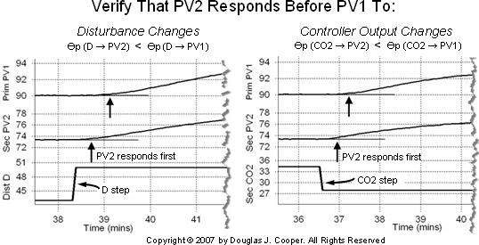
A successful cascade implementation requires that early warning process variable PV2 respond before outer primary PV1 both to changes in the jacket cooling liquid temperature disturbance (D) and to changes in inner secondary controller output signal CO2. The plots below (click for a large view) verify that both of these criteria are met with the architecture shown in the graphic above.
Expressed concisely, the plots show that the delay in response (or dead time, Өp) follows the rule:
Өp (D −› PV2) < Өp (D −› PV1) and Өp (CO2 −› PV2) < Өp (CO2 −› PV1)
Thus, a cascade control architecture should improve disturbance rejection performance relative to a single loop architecture.
P-Only vs. PI for Inner Secondary Controller
The cascade implementation recipe first helps us decide if the inner secondary controller is fast enough for a PI algorithm or if it is better suited for a P-Only algorithm. The decision is based on the size of the inner secondary time constant relative to that of the overall process time constant.
To compute these time constants, we need to bump the process and analyze the dynamic process response data. In this example we choose to place both inner secondary and outer primary controllers in manual mode (open loop) during the bump test. An alternative not explored here is to have the inner secondary controller in automatic mode with tuning sufficiently active to force a clear dynamic response in PV2.
Following the steps of the cascade implementation recipe:
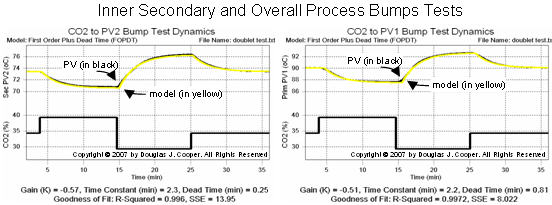
1) With the process steady at the design level of operation (DLO), we perform adoublet test, choosing here to move CO2 from 34.3% −› 39.3% −› 29.3% −› 34.3%. We record both PV2 and PV1 dynamic data as the process responds. We use this “step 1 data set” as we proceed with the implementation recipe.
2) As shown in the plots below, we use commercial software to fit a first order plus dead time (FOPDT) model to the inner secondary process (CO2 −› PV2) dynamic data and another to the overall process (CO2 −› PV1) dynamic data (click for a large view):
The FOPDT model parameters from these bump tests are summarized:
| Inner Secondary (CO2 −› PV2) |
Overall Process (CO2 −› PV1) |
|
| Process gain, Kp = | – 0.57 °C/% | – 0.51 °C/% |
| Time constant, Tp = | 2.3 min | 2.2 min |
| Dead time, Өp = | 0.25 min | 0.81 min |
The cascade block diagram implies that the time constant and dead time values for the inner process are contained within and contribute to the dynamics of the overall process. Thus, we can surmise that:
Tp (CO2 −› PV2) ≤ Tp (CO2 −› PV1) and Өp (CO2 −› PV2) ≤ Өp (CO2 −› PV1)
Yet the values in the table above indicate that this seemingly fundamental relationship does not hold true for the jacketed stirred reactor. In fact, when using a FOPDT model approximation of the dynamic response data, the time constant of the inner secondary process is slightly larger (longer) than that of the overall process.
The process graphic at the top of this article shows a main reactor vessel with a large volume of liquid relative to that of the cooling jacket. The function of the cooling jacket is to remove heat energy to regulate reactor vessel temperature. It seems logical that because of the volume differences, as long as the liquid temperature in the large reactor is changing, the temperature of the liquid in the small cooling jacket must follow. And the liquid in the reactor acts as a heat source because the chemical reaction inside the vessel generates heat energy faster as reactor temperature rises (and vice versa).
This intertwined relationship of heat generation and removal combined with relative sizes of the reactor and jacket offers one physical rationalization as to why the jacket (inner secondary) Tp might reasonably be longer than that of the vessel (overall process) Tp.
A simpler explanation is that the sensor used to measure temperature in the cooling jacket outlet flow was improperly specified at the time of purchase, and unfortunately, it responds slowly to actual cooling liquid changes. This additional response time alone could account for the observed behavior.
In any case, the dead time of the overall process is three times that of the inner secondary controller, and thus, PV2 provides a clear early warning that we can exploit for a cascade design. So while the simple cascade recipe has limitations that require our judgment, it provides valuable insights that enable us to proceed.
3) The cascade implementation recipe uses a time constant comparison to decide whether the inner secondary loop is fast enough for a PI controller. We reach a true statement with case 1 of the decision tree in step 3 of the recipe. That decision is:
if 3×Tp (CO2 −› PV2) > Tp (CO2 −› PV1) => Use P-Only controller
or using the parameters in the table above:
if 3(2.3 min) > 2.2 min => Use a P-Only controller
Inner Secondary Controller
4) Our cascade implementation recipe states that a P-Only algorithm is the best choice for the inner secondary controller. To explore this decision, we run four trials and compare P-Only and PI algorithms side-by-side. We are able to use the same “step 1 data set” for the design and tuning of all four of these inner secondary controllers:
TRIAL 1: moderate P-Only
TRIAL 2: aggressive P-Only
TRIAL 3: moderate PI
TRIAL 4: aggressive PI
As listed in the table in step 2 above, a first order plus dead time (FOPDT) model fit of the “step 1 data set” collected around our design level of operation (DLO) yields inner secondary FOPDT model parameters:
CO2 −› PV2 model: Kp = – 0.57 °C/%; Tp = 2.3 min; Өp = 0.25 min
Following our controller design and tuning recipe, we use these FOPDT model parameters in rules and correlations to complete the secondary controller design.
P-Only Controller design and tuning, including the use of the ITAE tuning correlation for computing controller gain, Kc, from FOPDT model parameters issummarized in the example in this article. Following those details:
TRIAL 1: Moderate P-Only TRIAL 2: Aggressive P-Only Kc = 2.5 (Moderate Kc) = 2.5 (–5.3) = – 13.3 %/oC PI Controller design and tuning, including computing controller gain, Kc, and reset time, Ti, from FOPDT model parameters is summarized in the example in this article. Following those details:
TRIAL 3: Moderate PI Moderate Tc = the larger of 1·Tp or 8·Өp
Aggressive Tc = the larger of 0.1·Tp or 0.8·Өp
|
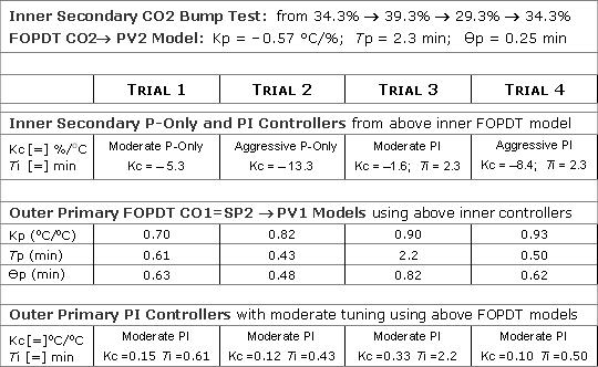
The “step 1 data set” model parameters and the four inner secondary controllers designed from this data are summarized in the upper half of the table below:
 |
Outer Primary Controller
5) We normally would implement one inner secondary controller and test it for acceptable performance. Here, we “accept” each of the four trial controllers and turn our attention to the outer primary loop.
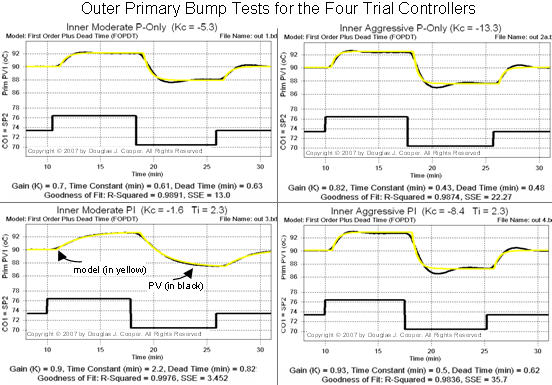
The four inner secondary controllers are thus implemented one after the other in a series of studies. When in automatic mode, each literally becomes part of the overall process. And because each is different, we must perform four separate bump tests and compute four sets of FOPDT model parameters to describe the four different outer primary (overall) dynamic process behaviors.
Recall that the output of the outer primary controller output, CO1, becomes the set point of the inner secondary controller, SP2. Thus, bumping CO1 is the same as bumping SP2 (i.e., CO1=SP2).
With each of the four inner secondary trial controllers in automatic, we choose to bump CO1=SP2 from 73.4 oC −› 76.4 oC −› 70.4 oC −› 73.4 oC. We again use commercial software to fit a FOPDT dynamic model to the CO1=SP2 −› PV2 dynamic response data sets as shown in the plots below (click for a large view). The FOPDT model parameters (Kp, Tp, Өp) from each bump test fit are summarized in the table above.
We find that industry practitioners, when designing a strategy for an application as challenging as reactor temperature control, generally seek a moderate response performance. Integral action will always be included to eliminate offset issues. Thus, we pair each inner secondary trial controller with a moderately tuned outer primary PI controller.
Following the identical procedure detailed in trial 3 of step 4 above, we compute four sets of moderate PI controller tuning parameters (one for each inner secondary controller). These are listed in the last row of the above table.
Compare Disturbance Rejection Performance
6) With both controllers in automatic, design and implementation of the cascade is complete. The objective of this cascade is to minimize the disruption to primary process variable PV1 when disturbance D changes.
The specific D of concern in this study is that the temperature of cooling liquid entering the jacket, normally at 43 oC, is known to spike occasionally to 50 oC.
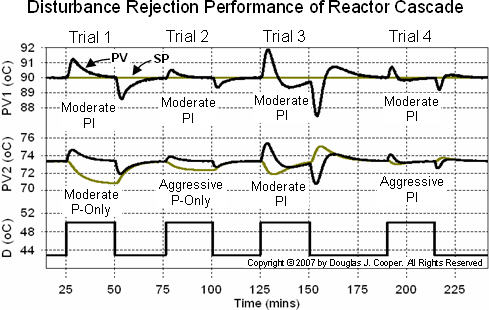
The lower trace in the plot below (click for a large view) shows disturbance steps (temperature changes) from 43 oC up to 50 oC and back. There are four trials shown, one for each of the inner secondary and outer primary controller pairs listed in the table above.
The middle portion of the plot shows the constantly moving inner secondary SP2=C01 in gold and the ability of early warning PV2 to track this ever-changing set point in black.
Recall that offset for early warning variable PV2 is not a concern in many cascade implementations. Here, for example, PV2 is cooling liquid temperature and cooling liquid is not a product destined for market. So our central focus is on how control actions based on this early warning variable help us minimize disturbance disruptions to PV1 and not on how precisely PV2 tracks set point.
Our success is shown on the upper portion of the plot. The outer primary set point, SP1 (in gold) remains constant throughout the study. Our interest is in the ability of each of the cascade implementations to maintain reactor exit temperature PV1 at SP1 in spite of the abrupt disturbance changes.
Some Observations
In general, a more successful (or “better”) cascade performance is one where:
▪ there is a smaller maximum deviation from set point during the disturbance, and
▪ PV1 most rapidly returns to and settles out at set point after a disturbance.
• Trials 2 and 4 both have aggressively tuned inner secondary controllers, and these two implementations both have the smallest deviations from set point and settle most rapidly back to SP. This supports the notion that inner secondary controllers should energetically attack early warning PV2 disruptions for best cascade performance.
• While an aggressively tuned inner secondary P-Only and PI controller (trials 2 and 4) performed with similar success, the moderately tuned inner secondary PI controller (trial 3) displayed markedly degraded performance. This high sensitivity to inner loop PI tuning strengthens the “use P-Only” conclusion made in step 3 of our cascade implementation recipe.
Comparing Cascade to Single Loop
The central question is whether the extra effort associated with cascade control provides sufficient payoff in the form of improved disturbance rejection performance.
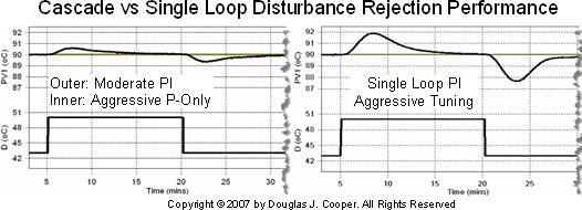
To the left in the plot below (click for a large view) is the performance of our trial 2 cascade implementation. The performance of an aggressively tuned single loop PI controller (design details in this article) in rejecting the same disturbance is shown to the right.
The cascade architecture reduces the maximum deviation from SP during the disturbance from ±2 oC for the single loop controller down to ±0.5 oC for the cascade. Settling time is shortened from about 10 minutes for the single loop controller down to about 8 minutes for the cascade.
If the financial return from such improved performance is greater than the cost to install and maintain the cascade, then choose cascade control.
Set Point Tracking Performance
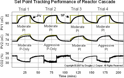
While not our design objective, presented below is the set point tracking performance of the four cascade implementations (click for a large view):
Cascade control is best suited for improved disturbance rejection. As shown above, its impact on set point tracking performance is minimal. While one might argue that our “best” cascade design for disturbance rejection (trial 2) also provides the most rapid SP tracking response, this same improvement can be obtained with more aggressive tuning of a single loop PI controller.


