By Bob Rice1 and Doug Cooper
Integrating (or non-self regulating) processes display counter-intuitive behaviors that make them surprisingly challenging to control. In particular, they do not naturally settle out to a steady operating level if left uncontrolled.
To address this distinctive dynamic character, we modify the controller design and tuning recipe to include a FOPDT Integrating model and slightly different design rules and tuning correlations as discussed here.
The Pumped Tank Process
To better understand the design and tuning of a PID controller for an integrating process, we explore the pumped tank case study from Control Station’s Loop-Prosoftware.
As shown below in manual mode (click for a large view), the process has two liquid streams feeding the top of the tank and a single exit stream pumped out the bottom.
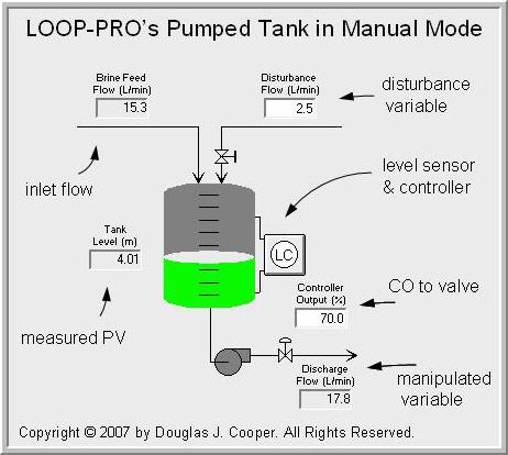
As labeled in the figure, the measured process variable (PV) is liquid level in the tank. To maintain level, the controller output (CO) signal adjusts a throttling valve at the discharge of a constant pressure pump to manipulate flow rate out of the bottom of the tank. This approximates the behavior of a centrifugal pump operating at relatively low throughput.
Unlike the gravity drained tanks case study where the exit flow rate increases and decreases as tank level rises and falls, the discharge flow rate here is strictly regulated by a pump. As a consequence, the physics do not naturally work to balance the system when any of the stream flow rates change.
This lack of a natural balancing behavior is why the pumped tank is classified as an integrating process. If the total flow into the tank is greater than the flow pumped out, the liquid level will rise and continue to rise until the tank fills or a stream flow changes. If the total flow into the tank is less than the flow pumped out, the liquid level will fall and continue to fall.
Below is a plot of the pumped tank behavior with the controller in manual mode (open loop). The CO signal is stepped up, increasing the discharge flow rate out of the bottom of the tank. The flow out becomes greater that the total feed into the top of the tank and as shown, liquid level begins to fall.
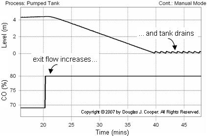
As the situation persists, liquid level continues to fall until the tank is drained. The saw-toothed effect shown when the tank is empty is because the pump briefly surges every time enough liquid accumulates for it to regain suction.
Not shown is that if the controller output were to be decreased enough to cause flow rate out to be less than flow rate in, the tank level would rise until full. If this were a real process, the tank would overflow and spill, creating safety and profitability issues.
The Disturbance Stream
As shown in the process graphic at the top of this article, the disturbance variable is a flow rate of a secondary feed into the top of the tank. This disturbance flow (D) is controlled independently, as if by another process (which is why it is a disturbance to our process).
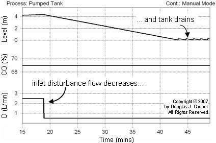
When D decreases (or increases), the measured PV level falls (or rises) in response. To illustrate, the plot below shows that the CO is held constant and D is decreased. Characteristic of an integrating process, the PV (tank level) starts falling because total flow into the tank is less than that pumped out. Like the case discussed above, the level continues to fall until the tank is drained.
Pumped Tank in Closed Loop
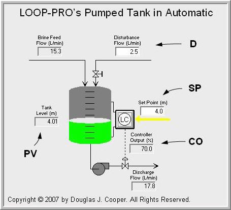
The process graphic below (click for a large view) shows the pumped tank in automatic mode (closed loop). The two streams feeding into the top of the tank total 17.8 L/min and level is steady because the controller regulates the discharge flow to this same value.
Graphical Modeling of Integrating Process Data
When collecting and analyzing data as detailed in steps 1 and 2 of the design and tuning recipe for integrating processes, we begin by specifying a design level of operation (DLO). In this study, we specify:
▪ Design PV = 4.8 m
▪ Design D = 2.5 L/min
Note that while not shown in the plots, D is held constant at 2.5 L/min throughout this study.
Just as with self regulating processes, step 3 of the recipe uses a simplifying dynamic model approximation to describe the complex behavior of a real process. The FOPDT Integrating model is simple in form yet it provides information sufficiently accurate for controller design and tuning.
The FOPDT Integrating model is:
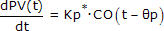
where the integrator gain, Kp*, has units of the ratio of the process gain to the process time constant, or:
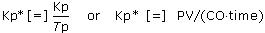
The graphical method of fitting a FOPDT Integrating model to process data requires a data set that includes at least two constant values of controller output, CO1 and CO2.
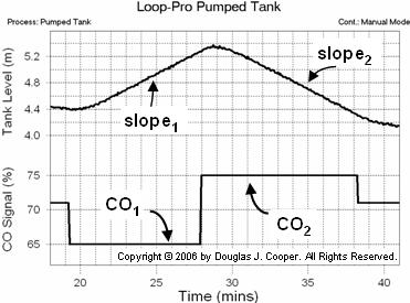
As shown below for the pumped tank, both must be held constant long enough so that a slope trend in the PV response (tank liquid level) can be visually identified.
An important difference between the graphical technique for self-regulating processesand integrating processes as discussed here is that integrating processes need not start at a steady value (steady-state) before a bump is made to the CO. The graphical technique discussed here is only concerned with the slopes (or rates of change) in PV and the controller output signal that caused each PV slope.
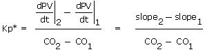
The FOPDT Integrating model describes the PV behavior at each value of constant controller output CO1 and CO2 as:
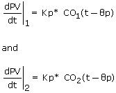
Subtracting and solving for Kp* yields:
Graphical Modeling of Pumped Tank Data
• Computing Integrator Gain
Below (click for a large view) is the same open loop data from the pumped tank simulation as shown above. The CO is stepped from 71% down to 65%, causing the liquid level (the PV) to rise. The controller output is then stepped from 65% up to 75%, causing a downward slope in the liquid level.
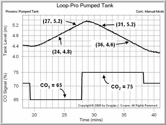
The slope of each segment is calculated as the change in tank liquid level divided by the change in time. From the plot data we compute:
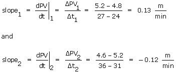
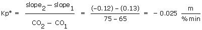
Using the two slopes computed above along with their respective CO values from the plot yields the integrator gain, Kp*, for the pumped tank:
• Computing Dead Time
The dead time is estimated from the plot using the same method described for the heat exchanger. That is, dead time, Өp, is computed as the difference in time from when the CO signal was stepped and when the measured PV starts a clear response to that change.
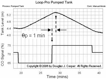
As shown above, the pumped tank dead time is estimated from the plot as:
Өp = 1.0 min
Thus, the FOPDT Integrator model information needed to proceed with controller tuning using the correlations presented here is complete.
Automating the Model Fit
In today’s world, there is no need to perform the model fit with graph paper and calculator. Commercial software offers analysis tools that makes fitting an FOPDT Integrating model quite simple.
Below, Control Station’s Loop-Pro software is used to analyze the pumped tank data. As shown (click for a large view), the software displays the data as a plot that includes adjustable nodes and tie lines.
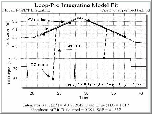
To compute a fit, click on the two CO nodes at the bottom of the plot and drag them to match the two values of constant controller output expected in the data. Both have tie lines to identify their associated PV slope bar. Each slope bar has two end point nodes. Click and drag these so that each bar approximates the sloping segments on the graph.
With the six nodes (two CO and four PV) properly positioned, the FOPDT Integrating model parameters are automatically calculated and the model fit is displayed over the raw data.
We can see that the model PV line matches the measured PV data, so we have confidence that the model fit is good. The image above also shows the FOPDT Integrator values computed by the software:
Kp* = – 0.023 m/(% min), Өp = 1.0 min
Recall that earlier in this article we computed by hand:
Kp* = – 0.025 m/(% min), Өp = 1.0 min
In the dynamic modeling world, these values are virtually identical. We note that software offers additional benefits in that it performs the computation quickly, reduces the chance of computational error, and provides a visual confirmation that the model used for controller design and tuning reasonably matches the process data.
PI Control Study
With bump test data centered around our design level of operation, and with an approximating FOPDT Integrating model of that data computed, we have completed steps 1-3 of the controller design and tuning recipe for this integrating process.
We complete the study by exploring PI control for the pumped tank process.
_______
1. Bob Rice holds primary responsibility at Control Station for training and software development, deployment, and support. Dr. Rice has published extensively on topics associated with automatic process control, including non-self-regulating processes and model predictive control. Prior to joining Control Station, Dr. Rice held engineering and technical positions with PPG Industries and The Walt Disney Company.
Robert Rice, Ph.D.
Director of Solutions Engineering
Control Station, Inc.
One Technology Drive
Tolland, CT 06084
Phone: (860) 872-2920
Email: bob.rice@controlstation.com
Web: http://www.controlstation.com