A controller seeks to maintain the measured process variable (PV) at set point (SP) in spite of unplanned and unmeasured disturbances. Since e(t) = SP — PV, this is equivalent to saying that a controller seeks to maintain controller error, e(t), equal to zero.
A controller repeats a measurement-computation-action procedure at every loop sample time, T. Starting at the far right of the control loop block diagram above (click for large view):
| ▪ | A sensor measures a temperature, pressure, concentration or other property of interest from our process. |
| ▪ | The sensor signal is transmitted to the controller. The pathway from sensor to controller might include: a transducer, an amplifier, a scaling element,quantization, a signal filter, a multiplexer, and other operations that can add delay and change the size, sign, and/or units of the measurement. |
| ▪ | After all electronic and digital operations, the result terminates at our controller as the “wire in” measured process variable (PV) signal. |
| ▪ | This “wire in” process variable is subtracted from set point in the controller to compute error, e(t) = SP — PV, which is then used in an algorithm (examples hereand here) to compute a controller output (CO) signal. |
| ▪ | The computed CO signal is transmitted on the “wire out” from the controller on a path to the final control element (FCE). |
| ▪ | Similar to the measurement path, the signal from the controller to FCE might include filtering, scaling, linearization, amplification, multiplexing, transducing and other operations that can add delay and change the size, sign, and/or units of our original CO signal. |
| ▪ | After any electronic and digital operations, the signal reaches the valve, pump, compressor or other FCE, causing a change in the manipulated variable (a liquid or gas stream flow rate, for example). |
| ▪ | The change in the manipulated variable causes a change in our temperature, pressure, concentration or other process property of interest, all with the goal of making e(t) = 0. |
Design Based on CO to PV Dynamics
The steps of the controller design and tuning recipe include: bumping the CO signal to generate CO to PV dynamic process data, approximating this test data with a first order plus dead time (FOPDT) model, and then using the model parameters in rules and correlations to complete the controller design and tuning.
The recipe provides a proven basis for controller design and tuning that avoids wasteful and expensive trial-and-error experiments. But for success, controller design and tuning must be based on process data as the controller sees it.
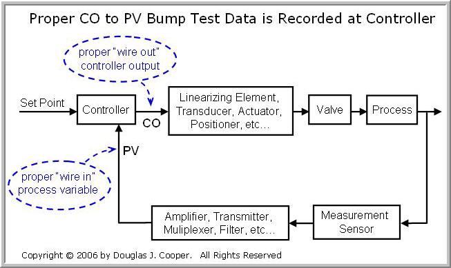
The controller only knows about the state of the process from the PV signal arriving on the “wire in” after all operations in the signal path from the sensor. It can only impact the state of the process with the CO signal it sends on the “wire out” before any such operations are made in the path to the final control element.
As indicated in the diagram at the top of this article, the proper signals that describe our complete “process” from the controller’s view is the “wire out” CO and the “wire in” PV.
Complete the Circuit
Sometimes we find ourselves unable to proceed with an orderly controller design and tuning. Perhaps our controller interface does not make it convenient to directly record process data. Maybe we find a vendor’s documentation to be so poorly written as to be all but worthless. There are a host of complications that can hinder progress.
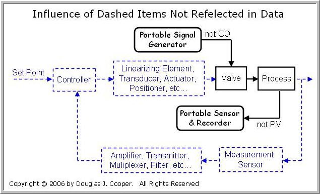
Being resourceful, we may be tempted to move the project forward by using portable instrumentation. It seems reasonable to collect, say, temperature in a vessel during a bump test by inserting a spare thermocouple into the liquid. Or maybe we feel we can be more precise by standing right at the valve and using a portable signal generator to bump the process rather than doing so from a remote control panel.
As shown below (click for large view), such an approach cuts out or short circuits the complete control loop pathway. External or portable instrumentation will not be recording the actual CO or PV as the controller sees it, and the data will not be appropriate for controller design or tuning.
Every Item Counts
The illustration above is extreme in that it shows many items that are not included in the control loop. But please recognize that it can be problematic to leave out even a single step in the complete signal pathway.
A simple scaling element that multiplies the signal by a constant value, for example, may seem reasonably unimportant to the overall loop dynamics. But this alone can change the size and even the sign of Kp, thus having dramatic impact on best tuning and final controller performance.
From a controller’s view, the complete loop goes from “wire out” to “wire in” as shown below.
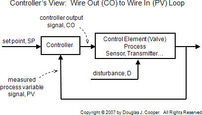
Every item in the loop counts. Always use the complete CO to PV data for process control analysis, design and tuning.
Pay Attention to Units
As detailed in this related article, signals can appear in a control loop in electronic units (e.g., volts, mA), in engineering units (e.g. oC, Lb/hr), as percent of scale (e.g., 0% to 100%), or as discrete or digital counts (e.g. 0 to 4095 counts).
It is critical that we remain aware of the units of a signal when working with a particular instrument or device. All values entered and computations performed must be consistent with the form of the data at that point in the loop.
Beyond the theory and methods discussed in this e-book, such “accounting confusion” can be one of the biggest challenges for the process control practitioner.