The same tuning recipe we successfully demonstrated for PI control and PID controldesign and tuning can be used when a controller output (CO) filter is added to the heat exchanger process control loop.
Here we explore PID with CO Filter control using the unified (controller with internal filter) form. We showed in this previous article that the unified form is identical to a PID with external first-order CO filter implementation. Hence, the methods we use and observations we make apply equally to both internal and external filter architectures.
We follow the same four-step design and tuning recipe used for all control implementations.
Steps 1-3 of the PID with CO Filter design are identical to our previous PI and PID control case studies. The details for steps 1-3, stated below as summary conclusions, are presented with discussion in the PI control study.
Step 1: Design Level of Operation (DLO)
▪ Design PV and SP = 138 °C with operation ranging from 138 to 140 °C
▪ Expected warm liquid flow disturbance = 10 L/min
Step 2: Collect Data at the DLO
See the PI control article referenced above for a summary, or go to this article to see details of the data collection experiment.
Step 3: Fit an FOPDT Model to the Dynamic Data
The first order plus dead time (FOPDT) model approximation of the heat exchanger data from step 2 is:
▪ Process gain (how far), Kp = –0.53 °C/%
▪ Time constant (how fast), Tp = 1.3 min
▪ Dead time (how much delay), Өp = 0.8 min
Step 4: Use the Parameters to Complete the Design
Vendors market the PID algorithm in a number of different forms, creating a confusing array of choices for the practitioner. The addition of a CO filter makes a bad situation worse. A filter adds another adjustable (tuning) parameter and significantly increases the number of possible algorithm forms.
Trial and error tuning of a four mode (four tuning parameter) controller with filter while our process is making product is a sure path to waste and expense. With so many interacting variables, we will likely settle for an operation that “isn’t horrible” rather than a performance that is near optimal.
The dilemma is real and our tuning recipe is the answer. Yet for success in this final step, it is critical that we match our algorithm with its proper tuning correlations.
The way to do this reliably is with loop tuning software. In fact, a good package will help with all of the steps, from data collection and model fitting through vendor algorithm selection and final performance analysis. When our task list includes maintaining and tuning loops during production, commercial software will pay for itself in days.
• Sample Time and Bumpless Transfer
As explained in the PI control study, best practice is to set loop sample time T ≤ 0.1Tp (10 times per time constant or faster). For this example, T = 1.0 sec.
Also, like most commercial controllers, we employ bumpless transfer. Thus, when switching to automatic, SP is set equal to the current PV and CObias is set equal to the current CO.
• Controller Action
Controller gain is negative for the heat exchanger, yet most commercial controllers require that a positive value of Kc be entered (more discussion here). The way we indicate a negative sign is to choose the direct acting option during implementation. If the wrong control action is entered, the controller will quickly drive the final control element to full on/open or full off/closed and remain there until a proper control action entry is made.
• Specify Desired Performance
We use the industry-proven Internal Model Control (IMC) tuning correlations in this study. IMC correlations employ a closed loop time constant, Tc, that describes the desired speed or quickness of our controller in responding to a set point change or rejecting a disturbance. We must decide whether we seek:
| ▪ | An aggressive controller with a rapid response and some overshoot: Tc is the larger of 0.1·Tp or 0.8·Өp |
| ▪ | A moderate controller that will move the PV reasonably fast yet produce little to no overshoot in a set point response: Tc is the larger of 1·Tp or 8·Өp |
| ▪ | A conservative controller that will move the PV in the proper direction, but quite slowly: Tc is the larger of 10·Tp or 80·Өp |
Ideal PID With Filter Example
A previous article presents details of how to combine an external first-order filter into a unified dependent, ideal, non-interacting PID with internal filter form:

If our vendor offers the option, the preferred algorithm in industrial practice is PID with derivative on measurement (derivative on PV).
While a CO filter can largely address derivative kick, the filter term must be made larger than otherwise necessary to do so. Thus, there remains a performance benefit to derivative on measurement even when using a CO filter.

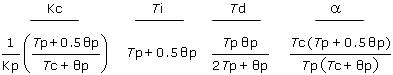
The IMC tuning correlations for either of the above PID with CO Filter forms are:
We start our study by choosing an aggressive response tuning:
Aggressive Tc = the larger of 0.1·Tp or 0.8·Өp
= larger of 0.1(1.3 min) or 0.8(0.8 min)
= 0.64 min
Using this Tc and our Kp, Tp and Өp from Step 3 in the tuning correlations above yields the aggressive PID w/ Filter tuning values below. Also listed are the PID Ideal and PI controller tuning values from earlier studies:
PID w/ Filter:
Kc = –2.2 %/°C Ti = 1.7 min Td = 0.31 min a = 0.6
PID:
Kc = –3.1 %/°C Ti = 1.7 min Td = 0.31 min
PI:
Kc = –1.7 %/°C Ti = 1.3 min
Below (click for large view) we compare the performance of these three aggressively tuned controllers side-by-side for the heat exchanger process simulation. Shown are three set point step pairs from 138 °C up to 140 °C and back again. Though not shown, the disturbance flow rate remains constant at 10 L/min throughout the study.
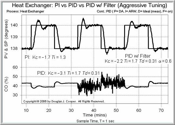
To the left is set point tracking performance for the PI controller. The middle set point steps show the performance of the PID controller. Derivative action enables a slightly faster rise time and settling time, but the derivative action causes the noise in the PV signal to be amplified and reflected as “chatter” in the control output signal.
To the right is the set point tracking performance of the PID w/ CO Filter controller. Indeed, the filter does an impressive job of cleaning up the chatter in the controller output signal without degrading performance.
In truth, however, the four tuning parameter PID w/ Filter performs similar to the two tuning parameter PI controller.
Tune One, Tune Them All
To complete this study, we compare the dependent, ideal, non-interacting form above to the performance of the dependent, interacting form:

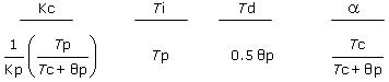
The tuning correlations for the dependent, interacting form are:
For variety, we choose moderate response tuning for this comparison:
Moderate Tc = the larger of 1·Tp or 8·Өp
= larger of 1(1.3 min) or 8(0.8 min)
= 6.4 min
Using this Tc and our model parameters in the proper tuning correlations, we arrive at these moderate tuning values:
Dependent, Interacting:
Kc = –0.34 %/°C Ti = 1.3 min Td = 0.40 min a = 0.9
Dependent, Ideal:
Kc = –0.44 %/°C Ti = 1.7 min Td = 0.31 min a = 1.2
As shown in the plot below (click for a large view), we see that moderate tuning provides a reasonably fast PV response while producing no overshoot. But more important, we establish that the interacting form and the ideal form provide identical performance when tuned with their own correlations.

The third set point step shows the performance of a straight PID with no filter. This reinforces the benefits of a CO filter if derivative action is being contemplated.
Observations
Our study of the heat exchanger process has shown that PID controllers provide minor performance improvements over PI controllers. Yet derivative action causes noise in the PV to be reflected as chatter in the CO signal, and this counterbalances the small benefits of the derivative term.
In this article, we explore CO filters and learn that they can correct the chatter problem. But now we have elevated a difficult two tuning parameter PI controller design into an extremely challenging four parameter PID w/ Filter controller design. And at best, this extra effort still provides only modest performance benefits.
Unless the economic impact of a loop is substantial, many practitioners conclude that the PI controller is the best choice. It is faster to implement, easier to maintain, and provides performance approaching that of the PID w/ Filter controller.
For the heat exchanger case study, this conclusion appears to be reasonable.