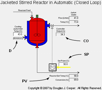
The control objective of the jacketed reactor case study, shown below and discussed in detailed in this article, is disturbance rejection. More specifically, we seek a controller design that will minimize the impact on reactor operation when the temperature of the liquid entering the cooling jacket changes.
As labeled in the graphic (click for large view), the important variables for this case study include:
CO = signal to valve that adjusts cooling jacket liquid flow rate (controller output, %)
PV = reactor exit stream temperature (measured process variable, oC)
SP = desired reactor exit stream temperature (set point, oC)
D = temperature of cooling liquid entering the jacket (major disturbance, oC)
Controller Design and Tuning Recipe
As with any control project, we follow our controller design and tuning recipe:
| 1. | Establish the design level of operation (the normal or expected values for set point and major disturbances) |
| 2. | Bump the process and collect controller output (CO) to process variable (PV) dynamic process data around this design level |
| 3. | Approximate the process data behavior with a first order plus dead time (FOPDT) dynamic model |
| 4. | Use the model parameters from step 3 in rules and correlations to complete the controller design and tuning. |
Step 1: Design Level of Operation (DLO)
The details and discussion for our DLO are presented in this article and are summarized:
▪ Design PV and SP = 90 oC with approval for brief dynamic testing of ±2 oC
▪ Design D = 43 oC with spikes up to 50 oC
Step 2: Collect Data at the DLO
The point of bumping a process is to generate and collect dynamic process data. To be of value, this data should be collected near our DLO and must clearly reveal the cause and effect relationship between how changes in the CO signal force a response in the measured PV.
• Data Must Be Wire Out to Wire In
The data must be collected from the controller’s viewpoint, since the controller will be making all decisions once in automatic mode. The controller only knows about the state of the process from the PV signal arriving on the “wire in” from the sensor. It can only impact the process with the CO signal it sends on the “wire out” to the final control element (e.g., a valve). All devices, mechanisms and instruments that affect the signal in the complete “wire-out to wire-in” CO to PV loop must be accounted for in the recorded data.
• Process Should Be Steady
To further isolate the pure cause and effect relationship, we should wait until the CO, PV and major disturbances have settled out and are reasonably constant before bumping the process. This provides us confidence that observed PV responses during the dynamic test are a direct result of the CO bumps. In the perfect world, this steady state will be at (or at least near) our DLO.
• Center Data Around the DLO
Like most processes with streams comprised of gases, liquids, powders, slurries and melts, the jacketed stirred reactor displays a nonlinear or changing behavior as operating level changes. In fact, it is this nonlinear character that leads us to specify a design level of operation in the first place. To the extent possible in our manufacturing environment, we should collect our process data centered around the DLO. A model fit of such data (step 3) will then average out the nonlinear effects and provide a controller equally balanced to address process movement both up and down.
• The PV Response Should Dominate the Noise
The CO bump must be far enough and fast enough to force a clear “cause and effect” response in the PV. And this PV response must clearly dominate the measurement noise.
Step 3: Fit a FOPDT Dynamic Model to Process Data Using Software
Two popular open loop (manual mode) methods for generating dynamic process response (bump test) data around the DLO include the step test and the doublet test. The primary disturbance (D) of interest in this study is cooling jacket inlet temperature. Not shown in the plots below is that D is steady at its design value of 43 oC during the bump tests.
| Practitioner’s Note: While the process graphic above shows the jacketed stirred reactor in automatic mode (closed loop), the step and doublet tests presented below are performed when the controller is in manual mode (open loop). |
◊ Step Test
Step tests have value because we can analyze the plot data by hand to compute the first order plus dead time (FOPDT) model parameters Kp, Tp and Өp. It is important that we have proper values for these model parameters because they are used in the rules and correlations of step 4 from the recipe to complete the controller design and tuning (examples here and here).
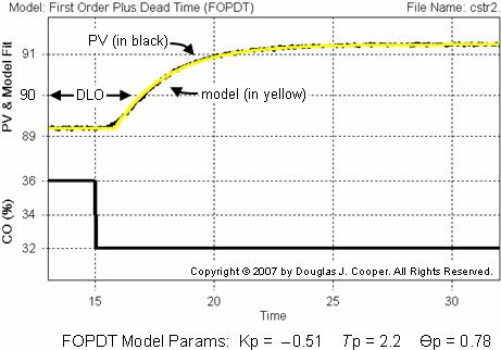
One disadvantage of a step test is that it is conducted in manual mode. As shown in the plot below, the PV is away from the DLO for an extended period of time. This can create profitability concerns from off-spec production and perhaps even safety concerns if constraints become violated.
To collect process data in manual mode that will “average out” the nonlinear effects around our design level of operation, we start the test at steady state with the PV on one side of the DLO. Then, as shown in the plot below, we step the CO so that the measured PV moves across to settle on the other side of the DLO.
We acknowledge that it may be unrealistic to attempt such a precise step test in some production environments. But we should understand that the motivation is to obtain an approximating FOPDT model of the dynamic response behavior that averages out the changing nature of the process as it moves across the expected range of operation.

A FOPDT model fit of the CO to PV data using commercial software is shown as the yellow trace in the plot above. It clearly tracks the measured PV data quite closely. The computed model parameters are listed below the plot.
Such results can be obtained in a few mouse clicks, and the visual confirmation that “model equals data” gives us confidence that we indeed have a meaningful description of the dynamic process behavior. This, in turn, gives us confidence that the subsequent controller design will provide the performance we desire.
◊ Doublet Test
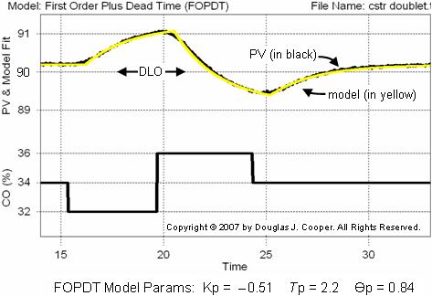
A doublet test, again performed below in manual mode, is two CO pulses made in rapid succession and in opposite direction. The second pulse is implemented as soon as the process has shown a clear response to the first pulse that dominates the noise in the PV. It is not necessary to wait for the process to respond to steady state for either pulse.

A FOPDT model fit of the CO to PV data using commercial software is shown as the yellow trace in the plot above. It also tracks the measured PV data quite closely.
A doublet test offers attractive benefits, including that:
▪ it starts from and quickly returns to the DLO,
▪ it produces data above and below the DLO to “average out” the nonlinear effects,
▪ the PV stays close to the DLO, minimizing off-spec production and safety concerns.
For these reasons, a doublet is preferred by many practitioners for open loop testing.
The FOPDT Model
By approximating the dynamic behavior of the jacketed reactor process with a first order plus dead time (FOPDT) model, we quantify those essential features that are fundamental to control.
Aside: the FOPDT dynamic model is a linear, ordinary differential equation describing how PV(t) responds over time to changes in CO(t):  Where in this case study: t [=] min, PV(t) [=] °C, CO(t – Өp) [=] % Where in this case study: t [=] min, PV(t) [=] °C, CO(t – Өp) [=] % |
The FOPDT model describes how the PV will respond to a change in CO with the:
▪ Process gain, Kp, that describes the direction and how far the PV will travel,
▪ Time constant, Tp, that states how fast the PV moves after it begins its response,
▪ Dead time, Өp, that is the delay that occurs from when CO is changed until when the PV begins its response.
Based on both the step and doublet test model fits shown above, we conclude that, when operating near the DLO, the jacketed reactor process dynamics are described:
• Kp = – 0.5 oC/%
• Tp = 2.2 min
• Өp = 0.8 min
We will use these parameter values in our subsequent control studies of the jacketed stirred reactor.


