Like the PI controller, the Proportional-Integral-Derivative (PID) controller computes a controller output (CO) signal for the final control element every sample time T.
The PID controller is a “three mode” controller. That is, its activity and performance is based on the values chosen for three tuning parameters, one each nominally associated with the proportional, integral and derivative terms.
As we had discussed previously, the PI controller is a reasonably straightforward equation with two adjustable tuning parameters. The number of different ways that commercial vendors can implement the PI form is fairly limited, and they all provide the same performance if properly tuned.
With the addition of a third adjustable tuning parameter, the number of algorithm permutations increases markedly. And there are even different forms of the PID equation itself. This creates added challenges for controller design and tuning.
Here we focus on what a derivative is, how it is computed, and what it means for control. We also explore why derivative on measurement is widely recommended for industrial practice.
We narrow our world in this article and focus on the dependent, ideal form of the controller. In later articles we will circle back and talk about the different algorithm forms, methods for design and tuning, algorithm limitations, and other practical issues.
The Dependent, Ideal PID Form
A popular way vendors express the dependent, ideal PID controller is:
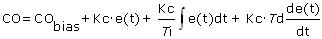
Where:
CO = controller output signal (the wire out)
CObias = controller bias; set by bumpless transfer
e(t) = current controller error, defined as SP – PV
SP = set point
PV = measured process variable (the wire in)
Kc = controller gain, a tuning parameter
Ti = reset time, a tuning parameter
Td = derivative time, a tuning parameter
The first three terms to the right of the equal sign are identical to the PI controller we have already explored in some detail.
The derivative mode of the PID controller is an additional and separate term added to the end of the equation that considers the derivative (or rate of change) of the error as it varies over time.
The Contribution of the Derivative Term
The proportional term considers how far PV is from SP at any instant in time. Its contribution to the CO is based on the size of e(t) only at time t. As e(t) grows or shrinks, the influence of the proportional term grows or shrinks immediately and proportionately.
The integral term addresses how long and how far PV has been away from SP. The integral term is continually summing e(t). Thus, even a small error, if it persists, will have a sum total that grows over time and the influence of the integral term will similarly grow.
A derivative describes how steep a curve is. More properly, a derivative describes the slope or the rate of change of a signal trace at a particular point in time. Accordingly, the derivative term in the PID equation above considers how fast, or the rate at which, error (or PV as we discuss next) is changing at the current moment.
Derivative on PV is Opposite but Equal
While the proportional and integral terms of the PID equation are driven by the controller error, e(t), the derivative computation in many commercial implementations should be based on the value of PV itself.
The derivative of e(t) is mathematically identical to the negative of the derivative of PV everywhere except when set point changes. And when set point changes, derivative on error results in an undesirable control action called derivative kick.
Math Note: the mathematical defense that “derivative of e(t) equals the negative derivative of PV when SP is constant” considers that, since e(t) = SP – PV, the equation below follows. That is, derivative of error equals derivative of set point minus process variable.The derivative of a constant is zero, so when SP is constant, mathematically, the derivative (or slope or rate of change) of the controller error equals the derivative (or slope or rate of change) of the measured process variable, PV, except the sign is opposite.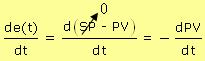 |
The figures below (click for a large view) provide a visual appreciation that the derivative of e(t) is the negative of the derivative of PV.
The top plot shows the measured PV trace after a set point step. The bottom plot shows the e(t) = SP – PV trace for the same event.
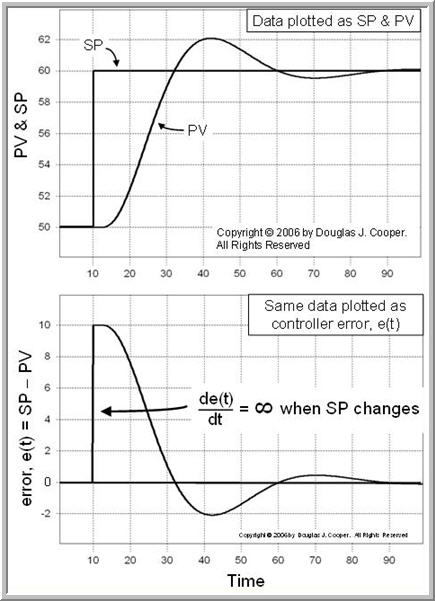
If we compare the two plots after the SP step at time t = 10, we see that the PV trace in the upper plot is an exact reflection of the e(t) trace in the lower plot. The PV trace ascends, peaks and then settles, while in a reflected pattern, the e(t) trace descends, dips and then settles.
Mathematically, this “mirror image” of trace shapes means that the derivatives (or slopes or rates of change) are the same everywhere after the SP step, except they are opposite in sign.
Derivative on PV Used in Practice
While the shape of e(t) and PV are opposite but equal everywhere after the set point step, there is an important difference at the moment the SP changes. The lower plot shows a vertical spike in e(t) at this moment. There is no corresponding spike in the PV plot.
The derivative (or slope) of a vertical spike in the theoretical world approaches infinity. In the real world it is at least a very big number. If Td is large enough to provide any meaningful weight to the derivative term, this huge derivative value will cause a large and sudden manipulation in CO. This large manipulation in CO, referred to as derivative kick, is almost always undesirable.
As long as loop sample time, T, is properly specified, the PV trace will follow a gradual and continuous response, avoiding the dramatic vertical spike evident in the e(t) trace.
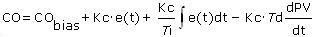
Because derivative on e(t) is identical to derivative on PV at all times except when the SP changes, and when the set point does change, derivative on error provides information we don’t want our controller to use, we substitute the “math note” equation in the yellow box above to obtain the PID with derivative on measurement controller:
Derivative on PV Does Not “Kick”
Below we show the heat exchanger case study under PID control using the dependent, ideal algorithm form and moderate tuning values as computed in this article.
The first set point steps to the left in the plot below (click for a large view) show loop performance when PID with derivative on error is used. The set points steps to the right present the identical scenario except that PID with derivative on measurement is used.
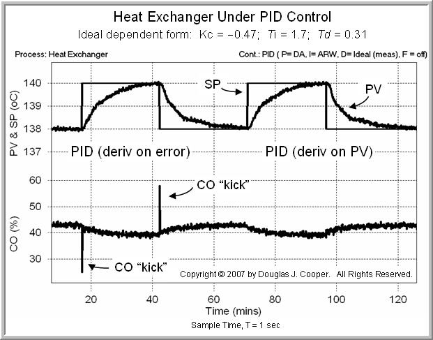
The “kick” that dominates the CO trace when derivative on error is used is rather dramatic and somewhat unsettling. While it exists for only a brief moment and does not impact performance in this example, we should not assume this will always be true. In any event, such action will eventually take a toll on mechanical final control elements.
Based on the preceding discussion, we recommend that derivative on measured PV be used if our vendor provides the option (fortunately most do). The tuning values remain the same for both algorithms.
Understanding Derivative Action
A rapidly changing PV has a steep slope and this yields a large derivative. This is true regardless of whether a dynamic event has just begun or if it has been underway for some time.
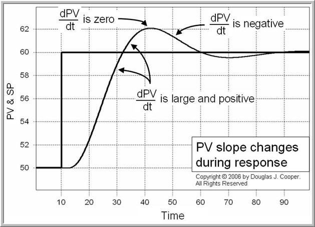
In the plot below (click for a large view), the derivative dPV/dt describes the slope or “steepness” of PV during a process response.
Early in the response, the slope is large and positive when the PV trace is increasing rapidly. When PV is decreasing, the derivative (slope) is negative. And when the PV goes through a peak or a trough, there is a moment in time when the derivative is zero.
To understand the impact of this changing derivative, let’s assume for discussion that:
| ▪ | Controller gain, Kc, is positive. |
| ▪ | Derivative time, Td (always positive) is large enough to provide meaningful weight to the derivative term. After all, if Td is very small, the derivative term has little influence, regardless of the slope of the PV. |
The negative sign in front of the derivative term of the PID with derivative on measurement controller (and given the above assumptions) means that the impact on CO from the derivative term will be opposite to the sign of the slope:
Thus, when dPV/dt is large and positive, the derivative term has a large influence and seeks to decrease CO.
Conversely, when dPV/dt is negative, the derivative term seeks to increase CO.
It is interesting to note that the derivative term does not consider whether PV is heading toward or away from the set point (whether e(t) is positive or negative). The only consideration is whether PV is heading up or down and how quickly.
The result is that derivative action seeks to inhibit rapid movements in the PV. This could be an especially useful characteristic when seeking to dampen the oscillations in PV that integral action tends to magnify. Unfortunately, as we will discuss, the potential benefit comes with a price.