We introduced the gravity drained tanks process in a previous article and established that it displays a self regulating behavior. We also learned that it exhibits a nonlinear behavior, though to a lesser degree than that of the heat exchanger.
Our control objective is to maintain liquid level in the lower tank at set point in spite of unplanned and unmeasured disturbances. The controller will achieve this by manipulating the inlet flow rate into the upper tank.
To proceed, we follow our controller design and tuning recipe:
| 1. | Establish the design level of operation (DLO), defined as the expected values for set point and major disturbances during normal operation |
| 2. | Bump the process and collect controller output (CO) to process variable (PV) dynamic process data around this design level |
| 3. | Approximate the process data behavior with a first order plus dead time (FOPDT) dynamic model to obtain estimates for process gain, Kp (how far variable), process time constant, Tp (how fast variable), and the process dead time, Өp (with how much delay variable). |
| 4. | Use the model parameters from step 3 in rules and correlations to complete the controller design and tuning. |
Step 1: Design Level of Operation (DLO)
Nonlinear behavior is a common characteristic of processes with streams comprised of liquids, gases, powders, slurries and melts. Nonlinear behavior implies that Kp, Tp and/or Өp changes as operating level changes.
Since we use Kp, Tp and Өp values in correlations to complete the controller design and tuning, the fact that they change gives us pause. It implies that a controller tuned to provide a desired performance at one operating level will not give that same performance at another level. In fact, we demonstrated this on the heat exchanger.
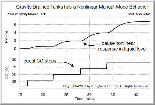
The nonlinear nature of the gravity drained tanks process is evident in the manual mode (open loop) response plot below (click for a larger view).

As shown, the CO is stepped in equal increments, yet the response (and thus the Kp,Tp, and/or Өp) changes as the level in the tank rises.
We address this concern by specifying a design level of operation (DLO) as the first step of our controller design and tuning recipe. If we are careful about how and where we collect our test data, we heighten the probability that the recipe will yield a controller with our desired performance.
The DLO includes where we expect the set point, SP, and measured process variable, PV, to be during normal operation, and the range of values the SP and PV might assume so we can explore the nature of the process across that range.
For the gravity drained tanks, the PV is liquid level in the lower tank. For this control study, we choose:
▪ Design PV and SP = 2.2 m with range of 2.0 to 2.4 m
The DLO also considers our major disturbances. We should know the normal or typical values for our major disturbances and be reasonably confident that they are quiet so we may proceed with a dynamic (bump) test.
The gravity drained tanks process has one major disturbance variable, the pumped flow disturbance, D. For this study, D is normally steady at about 2 L/min, but certain operations in the plant cause it to momentarily spike up to 5 L/min for brief periods.
Rejecting this disturbance is a major objective in our controller design. For this study, then:
▪ Design D = 2 L/min with occasional spikes up to 5 L/min
Step 2: Collect Data at the DLO (Design Level of Operation)
The next step in our recipe is to collect dynamic process data as near as practical to our design level of operation. We do this with a bump test, where we step or pulse the CO and collect data as the PV responds.
It is important to wait until the CO, PV and D have settled out and are as near to constant values as is possible for our particular operation before we start a bump test. The point of bumping a process is to learn about the cause and effect relationship between the CO and PV.
With the process steady, we are starting with a clean slate and as the PV responds to the CO bumps, the dynamic cause and effect behavior is isolated and evident in the data. On a practical note, be sure the data capture routine is enabled before the initial bump so all relevant data is collected.
While closed loop testing is an option, here we consider two open loop (manual mode) methods: the step test and the doublet test.
For either method, the CO must be moved far enough and fast enough to force a response in the PV that dominates the measurement noise.
Also, our bump should move the PV both above and below the DLO during testing. With data from each side of the DLO, the FOPDT model will be able to average out the nonlinear effects.
- Step Test
To collect data that will “average out” to our design level of operation, we start the test with the PV on one side of (either above or below) the DLO. Then, we step the CO so that the measurement moves across to settle on the other side of the DLO.
We acknowledge that it may be unrealistic to attempt such a precise step test in some production environments. But we should understand why we propose this ideal approach (answer: to average nonlinear process effects).
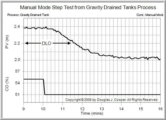
Recall that our DLO is a PV = 2.2 m and D = 2 L/min (though not shown on the plots, disturbance D remains constant at 2 L/min throughout the test).
Below, we set CO = 55% and the process steadies at a PV = 2.4 L.
Then, as shown below (click for a large view), we step the CO to 51% and the PV settles at abut 2.0 L/min. Thus, we have collected data “around” our design level of operation.

Note that we can start high and step the CO down (as above), or start low and step the CO up. Both methods produce dynamic data of equal value for our design and tuning recipe.
- Doublet Test
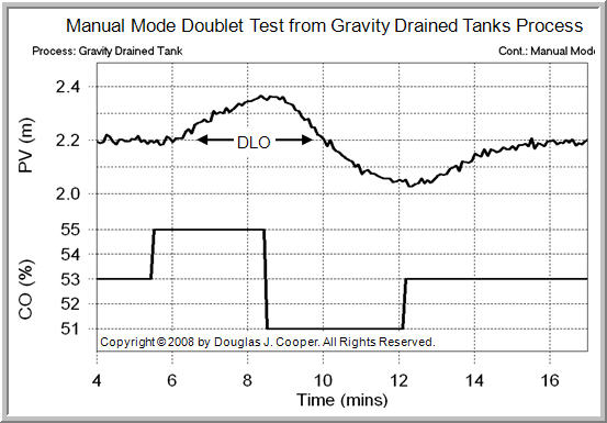
A doublet test, as shown below (click for a large view), is two CO pulses performed in rapid succession and in opposite direction.

The second pulse is implemented as soon as the process has shown a clear response to the first pulse that dominates the noise in the PV. It is not necessary to wait for the process to respond to steady state for either pulse.
The doublet test offers important benefits. Specifically, it:
| ▪ | starts from and quickly returns to the design level of operation, |
| ▪ | produces data both above and below the design level to “average out” the nonlinear effects, and |
| ▪ | the PV always stays close to the DLO, thus minimizing off-spec production. |
For these reasons, many industrial practitioners find the doublet to be the preferred method for generating open loop dynamic process data, though it does require that we use a commercial software tool for the model fitting task.
Modeling Process Dynamics
Next, we model the dynamics of the gravity drained tanks process and use the result in a series of control studies.