A valve cannot open more than all the way. A pump cannot go slower than stopped. Yet an improperly programmed control algorithm can issue such commands.
Herein lies the problem of integral windup (also referred to as reset windup or integral saturation). It is a problem that has been around for decades and was solved long ago. We discuss why it occurs and how to prevent it to help those who choose to write their own control algorithm.
The PI Algorithm
To increase our comfort level with the idea that different vendors cast the same PI algorithm in different forms, we choose the independent, continuous, position PI form for this discussion:
![]()
Where:
CO = controller output signal (the wire out)
CObias = controller bias or null value
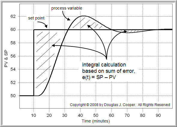
e(t) = current controller error, defined as SP – PV
SP = set point
PV = measured process variable (the wire in)
Kc = proportional gain, a tuning parameter
Ki = integral gain, a tuning parameter
Note that Kc is the same parameter in both the dependent and independent forms, though it is more typically called controller gain in the dependent form.
Every procedure and observation we have previously discussed about PI controllers applies to both forms. Both even use the same tuning correlations. To tune Ki, wecompute Kc and Ti for the dependent form and then divide (Ki = Kc/Ti).
Integral (Reset) Windup
Our previous discussion of integral action noted that integration is a continual summing. As shown below (click for a large view), integration of error means that we continually sum controller error up to the present time.

The integral sum starts accumulating when the controller is first put in automatic and continues to change as long as controller error exists.
If an error is large enough and/or persists long enough, it is mathematically possible for the integral term to grow very large (either positive or negative):
This large integral, when combined with the other terms in the equation, can produce a CO value that causes the final control element (FCE) to saturate. That is, the CO drives the FCE (e.g. valve, pump, compressor) to its physical limit of fully open/on/maximum or fully closed/off/minimum.
And if this extreme value is still not sufficient to eliminate the error, the simple mathematics of the controller algorithm, if not jacketed with protective logic, permits the integral term to continue growing.
If the integral term grows unchecked, the equation above can command the valve, pump or compressor to move to 110%, then 120% and more. Clearly, however, when an an FCE reaches its full 100% value, these last commands have no physical meaning and consequently, no impact on the process.
Control is Lost
Once we cross over to a “no physical meaning” computation, the controller has lost the ability to regulate the process.
When the computed CO exceeds the physical capabilities of the FCE because the integral term has reached a large positive or negative value, the controller is suffering fromwindup. Because windup is associated with the integral term, it is often referred to asintegral windup or reset windup.
To prevent windup from occurring, modern controllers are protected by either:
 |
Employing extra “jacketing logic” in the software to halt integration when the CO reaches a maximum or minimum value. |
| |
Recasting the controller into a discrete velocity form that, by its very formulation, naturally avoids windup. |
| Both alternatives offer benefits but possess some fairly subtle drawbacks that we discuss below. | |
Visualizing Windup
To better visualize the problem of windup and the benefit of anti-windup protection, consider the plot from our heat exchanger process below (click for a large view).
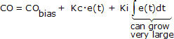
To the left is the performance of a PI controller with no windup protection. To the right is the performance of the same controller protected by an anti-windup strategy.
For both controllers, the set point is stepped from 200 °C up to 215 °C and back again. As shown in the lower trace on the plot, the controller moves the CO to 0%, closing the valve completely, yet this is not sufficient to move the PV up to the new set point.
To the left in the plot, the impact of windup is a degraded controller performance. When the set point is stepped back to its original value of 200 °C , the windup condition causes a delay in the CO action. This in turn causes a delay in the PV response.
To the right in the plot, anti-windup protection permits the CO, and thus PV, to respond promptly to the command to return to the original SP value of 200 °C.
More Details on Windup
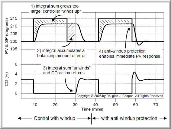
The plot below (click for large view) offers more detail. As labeled on the plot:
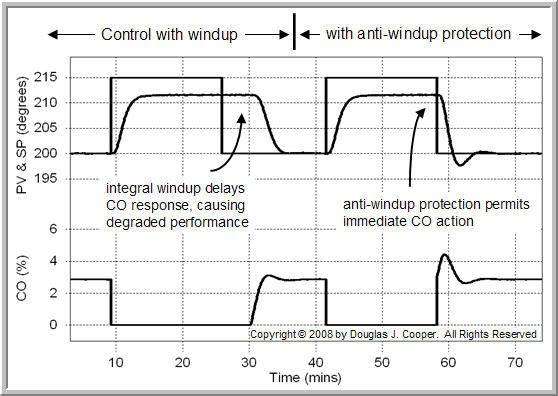
| 1) To the left for the Controller with Wind-up case, the SP is stepped up to 215 °C. The valve closes completely but is not able to move the PV all the way to the high set point value. Integration is a summing of controller error, and since error persists, the integration term grows very large. |
| The sustained error permits the controller to windup (saturate). While it is not obvious from the plot, the PI algorithm is computing values for CO that ask the valve to be open –5%, –8% and more. The control algorithm is just simple math with no ability to recognize that a valve cannot be open to a negative value. |
| Note that the chart shows the CO signal bottoming out at 0% while the controller algorithm is computing negative CO values. This misleading information is one reason why windup can be difficult to diagnose as the root cause of a problem from visual inspection of process data trend plots. |

| 2) When the SP is stepped back to 200 °C, it seems as if the CO does not move at first. In reality, the control algorithm started moving the CO when the SP changed, but the values remain in the physically meaningless range of negative numbers. |
| So while the valve remains fully closed at 0%, the integral sum is accumulating controller errors of opposite sign. As time passes, the integral term shrinks or “unwinds” as the running sum of errors balance out. |
| 3) When the integral sum of errors shrinks enough, it no longer dominates the CO computation. The CO signal returns from the physically meaningless world of negative values. The valve can finally move in response. |
| 4) To the right in the plot above, the controller is protected from windup. As a result, when the set point is stepped back to 200 °C, the CO immediately reacts with a change that is proportional to the size of the SP change. The PV moves quickly in response to the CO actions as it tracks the SP back to 200 °C. |
◊ Solution 1: Jacketing Logic on the Position Algorithm
The PI controller at the top of this article is called the position form because the computed CO is a specific intermediate value between full on/open/maximum and closed/off/minimum. The continuous PI algorithm is specifying the actual position (e.g., 27% open, 64% of maximum) that the final control element (FCE) should assume.
- Simple Logic Creates Additional Problems
It is not enough to have logic that simply limits or clips the CO if it reaches a maximum (COmax) or minimum (COmin) value because this does nothing to check the growth of the integral sum of errors term.
In fact, such simple logic was used in the “control with windup” plots just discussed. The CO seems stuck at 0% and we are unaware that the algorithm is actually computing negative valve positions as described in item 1 above.
- Anti-Windup Logic Outline
When we switch from manual mode to automatic, we assume that we have initialized the controller using a bumpless transfer procedure. That is, at switchover, the integral sum of error is set to zero, the SP is set equal to the current PV, and the controller bias is set equal to the current CO (implying that COmin < CObias < COmax).Thus, there is nothing to cause CO to immediately change and “bump” our process at switchover.
One approach to creating anti-windup jacketing logic is to artificially manipulate the integral sum of error itself. With our controller properly initialized, the approach is to flip the algorithm around and back-calculate a value for the integral sum of error that will provide a desired controller output value (COdesired), or:
![]()
Note that COdesired can be different in different situations. For example,
|
We do not want tuning parameter adjustments to cause sudden CO movements that bump our process. So if tuning values have changed, COdesired is the value of CO from the previous loop calculation cycle. |
|
If the PI controller computes CO values that are above COmax or below COmin, then we must be concerned about windup and COdesired is set equal to the limiting COmaxor COmin value. |
The anti-windup logic followed at every loop sample time, T, is thus:
| 1) | If tuning parameters have changed since the last loop calculation cycle, then COdesired = current CO. Back calculate the integral sum of error so CO remains unchanged from the previous sample time. This prevents sudden CO bumps due to tuning changes. | |
| 2) | Update SP and PV for this loop calculation cycle. | |
| 3) | compute: | |
| 4) | If CO > COmax or if CO < COmin, then the anti-windup (integral desaturation) logic of step 5 is required. Otherwise, proceed to step 6. | |
| 5) | If CO > COmax, then CO = COdesired = COmax. if CO < COmin, then CO = COdesired = COmin. Back calculate the integral sum of error using our selected COdesired and save it for use in the next control loop calculation cycle. | |
| 6) | Implement CO | |
◊ Solution 2 – Use the Velocity (Discrete) Controller Form
Rather than computing a CO signal indicating a specific position for our final control element, an alternative is to compute a signal that specifies a change, ∆CO, from current position for the FCE. As explained below, this is called the velocity or discrete controller form.
We employ the dependent algorithm for this presentation, but the derivation that follows can be applied in an analogous fashion to the independent PI form. To derive the discrete velocity form, we must first write the continuous, position form of the PI controller to include the independent variable on the controller output, showing it properly as CO(t) to reflect that it changes with time:
![]()
Please note that this controller is identical to all dependent PI forms as presented in other articles in this e-book. The only difference is we are being more mathematically precise in our expression of CO(t).
- Deriving the Discrete Velocity Form
The first step in deriving the discrete form is to take the time derivative of the continuous form. In physics, the time derivative (rate of change) of a position is a velocity. This is why the final form of the PI controller we derive is often called the velocity form.Taking the derivative of the continuous PI controller above with respect to time yields:
![]()
Since CObias is a constant and the derivative of a constant is zero, then:
![]()
Removing this term from the equation results in:
![]()
If we assume discrete or finite difference approximations for the continuous derivatives, then the controller becomes:
![]()
where ei is the current controller error, ei-1 is the controller error at the previous sample time, T, and ∆ei = ei – ei-1.
Recognizing that loop sample time is T = ∆t, then the PI controller becomes:
![]()
Rearranging, we arrive at the discrete velocity form of the PI controller:
![]()
- Reason for Anti-Windup Protection
Discrete velocity algorithms compute a ∆CO that signals the FCE to move a specific distance and direction from its current position. As we can see from the PI controller form above, the computation does not keep track of the current FCE position, nor does it mathematically accumulate any integral sums.
In a sense, the accumulation of integration is stored in the final control element itself. If a long series of ∆CO moves are all positive, for example, the valve, pump or compressor will move toward its maximum value. And once the FCE reaches its maximum limit, any ∆CO commands to move further will have no impact because, as stated in the first sentences of this article, a valve cannot open more than all the way and a pump cannot go slower than stopped. It is the physical nature of the FCE itself that provides protection from over-accumulation (i.e., windup).
As long as the CO never reaches COmax or COmin, the continuous position and discrete velocity forms of the PI controller provide identical performance. A properly jacketed continuous position PI controller will also provide windup protection equal to the discrete velocity form. Implicit in these statements is that sample time,T, is reasonably fast and that T and the tuning values (Kc and Ti) are the same when comparing implementations.
● Concerns with Discrete Velocity PID
Unfortunately, the usefulness of the discrete velocity form is limited because the method suffers problems when derivative action is included. We find that we must take the derivative of a derivative, yielding a second derivative. A second derivative applied to data that contains even modest noise can produce nonsense results.
Some vendors implement this form anyway and include a signal filter and additional logic sequences to address the problem. Thus, even with the anti-windup benefits of a discrete velocity algorithm, we find the need to jacket the algorithm with protective logic.