A previous article presented the first order plus dead time (FOPDT) dynamic model and discussed how this model, when used to approximate the controller output (CO) to process variable (PV) behavior of proper data from our process, yields the all-important model parameters:


The previous articles also mentioned that these FOPDT model parameters can be used to determine PID tuning values, proper sample time, whether the controller should be direct or reverse acting, whether dead time is large enough to cause concern, and more.
A Hands-On Study
There is an old saying (a Google search shows a host of attributed authors) that goes something like this: I hear and I forget, I see and I remember, I do and I understand.
Since our goal is to understand, this means we must “do.” To that end, we take a hands-on approach in this case study that will help us appreciate what each FOPDT model parameter is telling us about our process and empower us to act accordingly as we explore best practices for controller design and tuning.
To proceed, we require a process we can manipulate freely. We start with a heat exchanger because they are common to a great many industries.
Heat Exchanger Process
The heat exchanger we will study is really a process simulation from commercial software. The simulation is developed from first-principles theory, so its response behavior is realistic. The benefit of a simulation is that we can manipulate process variables whenever and however we desire without risk to people or profit.
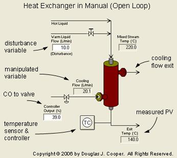
The heat exchanger is shown below (click for a large view) in manual mode (also called open loop). Its behavior is that of a counter-current, shell and tube, hot liquid cooler.
The measured process variable is the hot liquid temperature exiting the exchanger on the tube side. To regulate this hot exit temperature, the controller moves a valve to manipulate the flow rate of a cooling liquid entering on the shell side.
The hot tube side and cool shell side liquids do not mix. Rather, the cooling liquid surrounds the hot tubes and pulls off heat energy as it passes through the exchanger. As the flow rate of cooling liquid around the tubes increases (as the valve opens), more heat is removed and the temperature of the exiting hot liquid decreases.
A side stream of warm liquid combines with the hot liquid entering the exchanger and acts as a disturbance to our process in this case study. As the warm stream flow rate increases, the mixed stream temperature decreases (and vice versa).
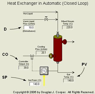
Shown below (click for a large view) is the heat exchanger in automatic mode (also called closed loop) using the standard nomenclature for this site.
The measured process variable (PV) is the hot liquid temperature exiting the exchanger. The controller output (CO) signal moves a valve to manipulate the flow rate of cooling liquid on the shell side to maintain the PV at set point (SP). The warm liquid flow acts as a disturbance (D) to the process.
Generating Step Test Data
To fit a FOPDT (first order plus dead time) model to dynamic process data using hand calculations, we will be reading numbers off of a plot. Such a graphical analysis technique can only be performed on step test data collected in manual mode (open loop).
| Practitioner’s Note: operations personnel can find switching to manual mode and performing step tests to be unacceptably disruptive, especially when the production schedule is tight. It is sometimes easier to convince them to perform a closed loop (automatic mode) pulse test, but such data must be analyzed by software and this reduces our “doing” to simply “seeing” software provide answers. |
To generate our dynamic process step test data, wait until the CO and PV appear to be as steady as is reasonable for the process under study. Then, after confirming we are in manual mode, step the CO to a new value.
The CO step must be large enough and sudden enough to cause the PV to move in a clear response that dominates all noise in the measurement signal. Data collection must begin before the CO step is implemented and continue until the PV reaches a new steady state.
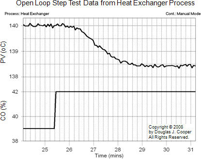
The plot below (click for a larger view) shows dynamic step test data from the heat exchanger. Note that the PV signal (the upper trace in the plot) includes a small amount of random measurement noise. This is added in the simulation to create a more realistic process behavior.
As shown in the plot, the CO is initially constant at 39% while the exit temperature PV is steady at about 140 °C. The CO is then stepped from 39% up to 42%.
The step increase in CO causes the valve to open, increasing the flow rate of cooling liquid into the shell side of the exchanger. The additional cooling liquid causes the measured PV (exit temperature on the tube side) to decrease from its initial steady state value of 140 °C down to a new value of about 138.4 °C.
We will refer back to the this dynamic process test data in future articles as we work through the details of computing process gain, Kp; process time constant, Tp; and process dead time, Өp.
| Practitioner’s Note: the heat exchanger graphic shows that this process has one disturbance variable, D. It is a side stream of warm liquid that mixes with the hot liquid on the tube side. When generating the step test data above, disturbance D is held constant.Yet real processes can have many disturbances, and by their very nature, disturbances are often beyond our ability to monitor, let alone control. While quiet disturbances are something we can guarantee in a simulation, we may not be so lucky in the plant. Yet to accurately model the dynamics of a process, it is essential that the influential disturbances remain quiet when generating dynamic process test data.Whether the disturbances have remained quiet during a dynamic test is something you must “know” about your process. Otherwise, you should not be adjusting any controller settings.
To appreciate this sentiment, recognize that you “know” when your car is acting up. You can sense when it shows a slight but clearly different behavior that needs attention. Someone planning to adjust the controllers in an industrial operation should have this same level of familiarity with their process. |


