Processes with streams comprised of gases, liquids, powders, slurries and melts tend to exhibit changing (or nonlinear) process behavior as operating level changes.
We discussed the nonlinear nature of the gravity drained tanks and heat exchanger processes in an earlier post. As we observed in that article and explore below, processes that are nonlinear with operating level will experience a degrading controller performance whenever the measured process variable (PV) moves away from the design level of operation (DLO).
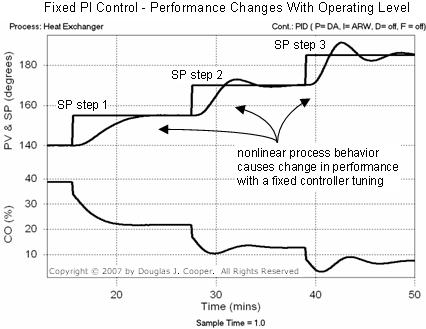
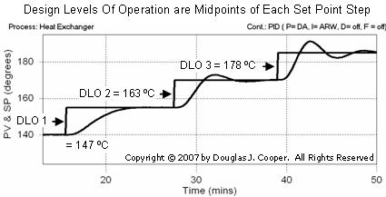
We demonstrate this problem on the heat exchanger running with a PI controller tuned for a moderate response. As shown in the first set point step from 140 °C to 155 °C in the plot below (click for large view), the PV responds in a manner consistent with our design goals. That is, the PV moves to the new set point (SP) in a deliberate fashion, but does not move so fast as to overshoot the set point.
The consequence of a nonlinear process behavior is apparent as the set point steps continue to higher temperatures. In the third SP step from 170 °C to 185 °C, the same PI controller that had given a desired moderate performance now produces an active PV response with a clear overshoot and slowly damping oscillations.
If we decide that such a change in performance with operating level is not acceptable, then parameter scheduled adaptive control may be an appropriate solution.
Developing an adaptive control strategy requires additional bump tests that may disrupt production. Once sufficient process data is collected, adaptive controller design and implementation consumes more personnel time. Before we start the project, we should be sure that the loop has sufficient impact on our profitability to justify the effort and expense.
Parameter Scheduled Adaptive Control
The method of approach for parameter scheduled adaptive control is to:
| a) | Divide the total range of operation into some number of discrete increments or operating ranges. |
| b) | Select a controller algorithm (P-Only, PI, PID or PID with CO Filter) for the application. |
| c) | Specify loop sample time, action of the controller (reverse or direct acting), and other design values that will remain constant in spite of nonlinear behavior. |
| d) | Apply our controller tuning recipe and compute tuning values for our selected controller at each of the operating increments as chosen in step a). |
We require a computer based control system (a DCS or advanced PLC) to implement the adaptive logic. This is because the tuning values must be programmed as a look-up table (or schedule) where the measured PV indicates the current level of operation, and as such, “points” to appropriate controller tuning values in the table at any moment in time.
Once online, the computer reads a set of tuning values from the table as indicated by the current value of the PV. These are downloaded into the controller algorithm, which then proceeds to calculate the next controller output (CO) value.
Tuning updates are downloaded into the controller every loop sample time, T. As a result, the controller continually adapts as the operating level changes to maintain a reasonably consistent control performance across a range of nonlinear behavior.
| Notes: 1) The set point (SP) is not appropriate to use as the operating level “pointer” because it indicates where we hope the PV will be, not necessarily where it actually is. The CO value can change both as operating level changes and as the controller works to reject disturbances. Since it reflects both disturbance load and operating level, the correspondence between current CO and current operating level is inconsistent. Current PV offers the most reliable indicator of expected process behavior. 2) “Gain scheduling” is a simplified variation of parameter scheduling, where, rather than updating all tuning values as operating level changes, only the controller gain is updated. All other tuning values remain constant with a pure gain scheduling approach. This simplification increases the chance that important process behaviors (such as a changing dead time, Өp) will be overlooked, thus decreasing the potential benefit of the adaptive strategy. With modern computing capability now widely available, we see no benefit from a “gain only” simplification unless it is the only choice offered by our vendor. |
Interpolation Saves Time and Money
Ultimately, it is impractical to divide our range of operation into many increments and then tune a controller at each level. Such an approach requires that we bump the process at least once in each operating increment. As we had alluded to in previous discussion, this can cause significant disruption to the production schedule, increase waste generation, use expensive materials and utilities, consume precious personnel time, and everything else that makes any loop tuning project difficult to sell in a production environment.
Thus, a popular variation on parameter scheduling, and the one explored in the case study below, is to design and tune only three controllers that span the range of expected operation. We then interpolate (fit a line) between the tuning values so we can update (or adapt) our controller to match any operating level at any time.
Normally, one controller is tuned to operate near the lower set point value we expect to encounter, while another is tuned for the expected high SP value. The third controller is then tuned for a strategically located mid range operation to give an appropriate shape to our interpolation curve. Our goal in choosing where to locate this midpoint is to reasonably approximate the complex nonlinear behavior of our process while keeping disruptive testing to a minimum. More discussion follows in the case study.
Case Study: Adaptive Control of the Heat Exchanger
We use the heat exchanger to illustrate and explore the ideas introduced above. As always, we follow our controller design and tuning recipe as we proceed. We choose a PI controller for the study and use the constant design values as detailed here (e.g., dependent PI algorithm form; loop sample time, T = 1.0 sec; controller is direct acting).
Step 1: Design Level of Operation (DLO)
Our adaptive schedule requires tuning values for three PI controllers that span the range of expected operation. Hence, we need to specify three design levels of operation (DLOs), one for each controller.
Since, as we detail here, set point driven data can be analyzed with commercial software for controller design and tuning, we will use the data from the plot at the top of this post as our bump test data.
As discussed in this article, a good bump test should generate dynamic process data both above and below the DLO. This is best practice because we then “average out” nonlinear effects when, in step 3 that follows, we approximate the bump test data with a simplifying first order plus dead time (FOPDT) dynamic model.
Since our test data has already been collected and plotted, we reverse this logic and pick the three DLOs as the midpoint of each SP step. Reading from the plot as shown below, we thus arrive at: DLO 1 = 147 °C; DLO 2 = 163 °C; DLO 3 = 178 °C
Step 2: Collect Process Data around the DLO
The plot data provides us with three complete CO to PV bump tests, each centered around its DLO. Hence, step 2 is complete.
Step 3: Fit a FOPDT Model to the Dynamic Process Data
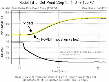
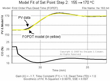
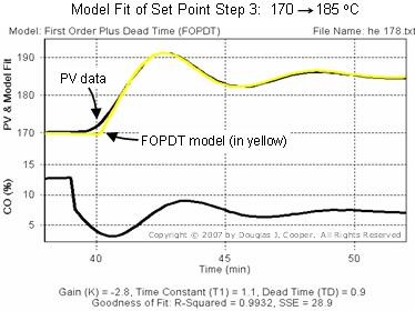
We use Control Station’s Loop-Pro software to divide the plot data into three CO to PV bump tests. We then use the software to fit a FOPDT model to each bump test following the same procedure as detailed here.
The plots below (see large view of step 1, step 2, or step 3) show the data and FOPDT model approximations. Because each FOPDT model visually matches its bump test data, we have confidence that the model parameters (listed below each plot and summarized in the table in Step 4) reasonably describe the dynamic process behavior at the three design levels of operation.
Step 4: Use the FOPDT Model Parameters to Complete the Design
The table below summarizes the FOPDT model parameters from step 3 for the three DLOs.
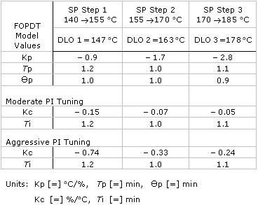
Note that the process gain, Kp, varies by 300% (from -0.9 to -2.8 °C/%) across the operating range. In contrast, process time constant, Tp, and process dead time, Өp, change by quite modest amounts.
For this investigation, we compute both moderate and aggressive PI tuning values for each DLO. The rules and correlations for this are detailed in this post, but briefly, we compute our closed loop time constant, Tc, as:
▪ aggressive: Tc is the larger of 0.1·Tp or 0.8·Өp
▪ moderate: Tc is the larger of 1·Tp or 8·Өp
With Tc computed, the PI correlations for controller gain, Kc, and reset time, Ti, are:

The moderate and aggressive PI tuning values for each of the DLOs are also summarized in the table above.
Below we illustrate how to interpolate controller gain, Kc, for the moderate tuning case.
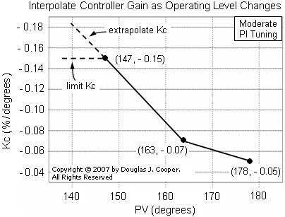
As shown in the plot, the three moderate Kc values are plotted as a function of PV. Lines of interpolation are fitted between each Kc value. The equations for these linesmust be programmed into the control computer.
Now, as PV moves anywhere from 147 to 178 oC, we can use these equations to compute a unique value for Kc. This concept must also be applied to obtain interpolating equations for reset time, Ti, thus producing a fully adaptive controller.
As shown in the plot above, one decision that must be made is whether to extrapolate the line and have the parameter continue the trend past the actual maximum or minimum data point. Alternatively, we could choose to limit Kc and have it stay constant for all PV values beyond the maximum or minimum.
Unless we are confident that we understand the true nature of a process, extrapolation into the unknown is more often a bad idea than a good one. In this case study, we choose not to extrapolate. Rather, we limit the tuning parameters to the maximum and minimum DLO values in the table. That is, Kc remains constant at -0.15 %/°C when PV moves below 147 oC, and remains constant at -0.05 when Kc moves above 178 oC. In between, Kc tracks the interpolating lines in the plot above.
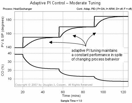
The capability of this parameter scheduled adaptive control is shown for a moderate PI controller in the plot below (click for large view). To appreciate the difference, compare this constant performance to the varied response in the plot at the top of this post.
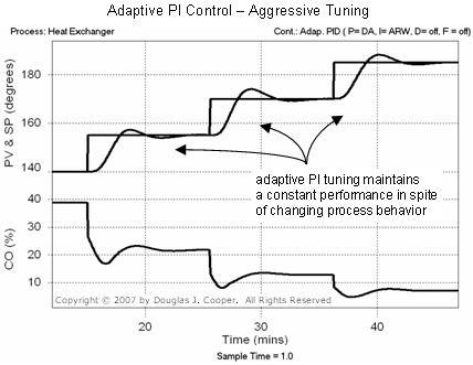
The result of an aggressively tuned PI controller is shown in the plot below (click for large view). The performance response is again quite consistent (though admittedly not perfect) across the range of operation.
A Proven Strategy
As these plots illustrate, a parameter scheduled adaptive controller can achieve consistent performance on processes that are nonlinear with operating level. This adaptive strategy has been widely employed in industrial practice and, as shown in this case study, is quite powerful in addressing a challenging and important problem.
Again, however, design and implementation requires extra effort and expense. We should be sure the loop is important enough to warrant such an investment before we begin.


