Automatic control systems enable us to operate our processes in a safe and profitable manner. Consider, as on this site, processes with streams comprised of gases, liquids, powders, slurries and melts. Control systems achieve this “safe and profitable” objective by continually measuring process variables such as temperature, pressure, level, flow and concentration – and taking actions such as opening valves, slowing down pumps and turning up heaters – all so that the measured process variables are maintained at operator specified set point values.
Safety First
The overriding motivation for automatic control is safety, which encompasses the safety of people, the environment and equipment.
The safety of plant personnel and people in the community are the highest priority in any plant operation. The design of a process and associated control system must always make human safety the primary objective.
The tradeoff between safety of the environment and safety of equipment is considered on a case by case basis. At the extremes, the control system of a multi-billion dollar nuclear power facility will permit the entire plant to become ruined rather than allow significant radiation to be leaked to the environment.
On the other hand, the control system of a coal-fired power plant may permit a large cloud of smoke to be released to the environment rather than allowing damage to occur to, say, a single pump or compressor worth a few thousand dollars.
The Profit Motive
When people, the environment and plant equipment are properly protected, our control objectives can focus on the profit motive. Automatic control systems offer strong benefits in this regard.
Plant-level control objectives motivated by profit include:
 meeting final product specifications
minimizing waste production
minimizing environmental impact
minimizing energy use
maximizing overall production rate
It can be most profitable to operate as close as possible to these minimum or maximum objectives. For example, our customers often set our product specifications, and it is essential that we meet them if failing to do so means losing a sale.
Suppose we are making a film or sheet product. It takes more raw material to make a product thicker than the minimum our customers will accept on delivery. Consequently, the closer we can operate to the minimum permitted thickness constraint without going under, the less material we use and the greater our profit.
Or perhaps we sell a product that tends to be contaminated with an impurity and our customers have set a maximum acceptable value for this contaminant. It takes more processing effort (more money) to remove impurities, so the closer we can operate to the maximum permitted impurity constraint without going over, the greater the profit.
Whether it is a product specification, energy usage, production rate, or other objective, approaching these targets ultimately translates into operating the individual process units within the plant as close as possible to predetermined set point values for temperature, pressure, level, flow, concentration and the other measured process variables.
Controllers Reduce Variability
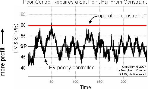
As shown in the plot below, a poorly controlled process can exhibit large variability in a measured process variable (e.g., temperature, pressure, level, flow, concentration) over time.
Suppose, as in this example, the measured process variable (PV) must not exceed a maximum value. And as is often the case, the closer we can run to this operating constraint, the greater our profit (note the vertical axis label on the plot).
To ensure our operating constraint limit is not exceeded, the operator-specified set point (SP), that is, the point where we want the control system to maintain our PV, must be set far from the constraint to ensure it is never violated. Note in the plot that SP is set at 50% when our PV is poorly controlled.
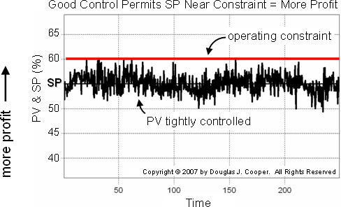
Below we see the same process with improved control. There is significantly less variability in the measured PV, and as a result, the SP can be moved closer to the operating constraint.
With the SP in the plot below moved to 55%, the average PV is maintained closer to the specification limit while still remaining below the maximum allowed value. The result is increased profitability of our operation.
Terminology of Control
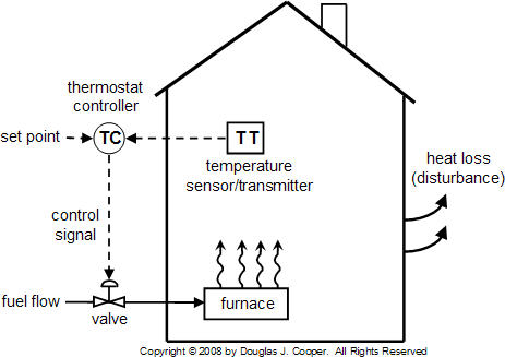
We establish the jargon for this site by discussing a home heating control system as illustrated below.
This is a simplistic example because a home furnace is either on or off. Most control challenges have a final control element (FCE), such as a valve, pump or compressor, that can receive and respond to a complete range of controller output (CO) signals between full on and full off. This would include, for example, a valve that can be open 37% or a pump that can be running at 73%.
For our home heating process, the control objective is to keep the measured process variable (PV) at the set point value (SP) in spite of unmeasured disturbances (D).
| For our home heating system: | |
| PV = | process variable is house temperature |
| CO = | controller output signal from thermostat to furnace valve |
| SP = | set point is the desired temperature set on the thermostat by the home owner |
| D = | heat loss disturbances from doors, walls and windows; changing outdoor temperature; sunrise and sunset; rain… |
To achieve this control objective, the measured process variable is compared to the thermostat set point. The difference between the two is the controller error, which is used in a control algorithm such as a PID (proportional-integral-derivative) controller to compute a CO signal to the final control element (FCE).
The change in the controller output (CO) signal causes a response in the final control element (fuel flow valve), which subsequently causes a change in the manipulated process variable (flow of fuel to the furnace). If the manipulated process variable is moved in the right direction and by the right amount, the measured process variable will be maintained at set point, thus satisfying the control objective.
This example, like all in process control, involves a measurement, computation and action:
is the measured temp colder than set point (SP – PV > 0)? Then open the valve.
is the measured temp hotter than set point (SP – PV < 0)? Then close the valve.
Note that computing the necessary controller action is based on controller error, or the difference between the set point and the measured process variable, i.e.
e(t) = SP – PV (error = set point – measured process variable)
In a home heating process, control is an on/off or open/close decision. And as outlined above, it is a straightforward decision to make. The price of such simplicity, however, is that the capability to tightly regulate our measured PV is rather limited.
One situation not addressed above is the action to take when PV = SP (i.e., e(t) = 0). And in industrial practice, we are concerned with variable position final control elements, so the challenge elevates to computing:
the direction to move the valve, pump, compressor, heating element…
how far to move it at this moment
how long to wait before moving it again
whether there should be a delay between measurement and action
This site
This site offers information and discussion on proven methods and practices for PID (proportional-integral-derivative) control and related architectures such as cascade, feed forward, Smith predictors, multivariable decoupling, and similar traditional and advanced classical strategies.
Applications focus on processes with streams comprised of gases, liquids, powders, slurries and melts. As stated above, final control elements for these applications tend to be valves, variable speed pumps and compressors, and cooling and heating elements.
Industries that operate such processes include chemical, bio-pharma, oil and gas, paints and coatings, food and beverages, cement and coal, polymers and plastics, metals and materials, pulp and paper, personal care products, and more.