When considering the range of control challenges found across the process industries, it becomes apparent that very different controller behaviors can be considered “good” performance. While one process may be best operated with a fast and aggressive control action, another may be better suited for a slow and gentle response.
Since there is no common definition of what is good or best performance, we are the judge and jury of goodness for our own process.
Performance is a Matter of Application
Suppose our process throughput is known to change quite suddenly because of the unreliable nature of our product filling/packaging stations at the end of our production line. When one of the container filling stations goes down, the upstream process throughput must be ramped down quickly to compensate. And as soon as the problem is corrected, we seek to return to full production as rapidly as possible.
In this application, we may choose to tune our controllers to respond aggressively to sudden changes in throughput demand. We must recognize and accept that the consequence of such aggressive action is that our process variables (PVs) may overshoot and oscillate as they settle out after each event.
Now suppose we work for a bio-pharma company where we grow live cell cultures in large bioreactors. Cells do not do well and can even die when conditions change too quickly. To avoid stressing the culture, it is critical that the controllers move the process variables slowly when they are counteracting disturbances or working to track set point changes.
So good performance can sometimes mean fast and aggressive, and other times slow and gentle.
Sometimes Performance is a Matter of Location
Distillation columns are towers of steel that can be as tall as a 20 story building. They are designed to separate mixtures of liquids into heavier and lighter components. To achieve this, they must run at precise temperatures, pressures and flow rates.
Because of their massive size, they have time constants measured in hours. A disturbance upset in one of the these behemoths can cause fluctuations (called “swings”) in conditions that can take the better part of a day to settle out. If the plant is highly integrated with streams coming and going from process units scattered across the facility, then a distillation column swinging back and forth for hours will cause the operation of units throughout the plant to be disrupted.
So the rule of thumb in such an integrated operation is that the columns are king. If we are involved in operating a process upstream of a distillation column, we do everything in our power to contain all disruptions within our unit. Good control means keeping our problems to ourselves and avoiding actions that will impact the columns. We do this no matter what havoc it creates for our own production.
And if we are involved in operating a process downstream from a column, our life can be similarly miserable. The column controllers are permitted to take whatever action is necessary to keep the columns running smoothly. And this means that streams flowing out of the column can change drastically from moment to moment as the controllers fight to maintain balance.
A Performance Checklist
As these examples illustrate, good control performance is application specific. Ultimately, we define “best” based on our own knowledge and experience. Things we should take into account as we form our judgments include what our process is physically able to achieve, how this fits into the bigger safety and profitability picture of the facility, and what management has planned.
Thus, our performance checklist requires consideration of the:
▪ goals of production
▪ capabilities of the process
▪ impact on down stream units
▪ desires of management
Controller Performance from Plot Data
If we limit ourselves to judging the performance of a specific controller on one of our own processes, we can compare response plots side-by-side and make meaningful statements about which result is “better” as we define it.
There are more precise terms beyond “oscillates a lot” or “responds quickly.” We explore below several criteria that are computed directly from plot data. The more common terms in this category include:
▪ rise time
▪ peak overshoot ratio
▪ settling time
▪ decay ratio
These and like terms permit us to make orderly comparisons among the range of performance available to us.
Peak Related Criteria
Below is a set point step response plot (click for a larger view) with labels indicating peak features:
A = size of the set point step
B = height of the first peak
C = height of the second peak
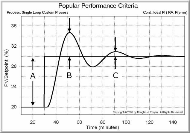
The popular peak related criteria include:
• Peak Overshoot Ratio (POR) = B/A
• Decay Ratio = C/B
In the plot above, the PV was initially at 20% and a set point step moves it to 30%. Applying the peak related criteria by reading off the PV axis:
A = (30 – 20) = 10%
B = (34.5 – 30) = 4.5%
C = (31 – 30) = 1%
And so for this response:
POR = 4.5/10 = 0.45 or 45%
Decay ratio = 1/4.5 = 0.22 or 22%
An old rule of thumb is that a 10% POR and 25% decay ratio (sometimes called a quarter decay) are popular values. Yet in today’s industrial practice, many plants require a “fast response but no overshoot” control performance.
No overshoot means no peaks, and thus, B = C = 0. This increasingly common definition of “good” performance means the peak related criteria discussed above are not useful or sufficient as performance comparison measures.
Time Related Criteria
An additional set of measures focus on time-related criteria. Below is the same set point response plot (click for a larger view) but with the time of certain events labeled:
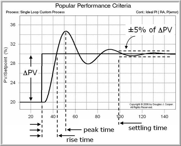
The clock for time related events begins when the set point is stepped, and as shown in the plot, include:
• Rise Time = time until the PV first crosses the set point
• Peak Time = time to the first peak
• Settling Time = time to when the PV first enters and then remains within a band whose width is computed as a percentage of the total change in PV (or DPV).
The 5% band used to determine settling time in the plot above was chosen arbitrarily. As we will see below, other percentages are equally valid depending on the situation.
From the plot, we see that the set point is stepped at time t = 30 min. The time related criteria are then computed by reading off the time axis as:
Rise Time = (43 – 30) = 13 min
Peak Time = (51 – 30) = 21 min
Settling Time = (100 – 30) = 70 min for a ±5% of DPV band
When There is No Overshoot
We should recognize that the peak and time criteria are not independent:
▪ a process with a large decay ratio will likely have a long settling time.
▪ a process with a long rise time will likely have a long peak time.
And in situations where we seek moderate tuning with no overshoot in our response plots, there is no peak overshoot ratio, decay ratio or peak time to compute. Even rise time, with its asymptotic approach to the new steady state, is a measure of questionable value.
In such cases, settling time, or the time to enter and remain within a band of width we choose, still remains a useful measure.
The plot below (click for a larger view) shows the identical process as that in the previous plots. The only difference is that in this case, the controller is tuned for a moderate response.
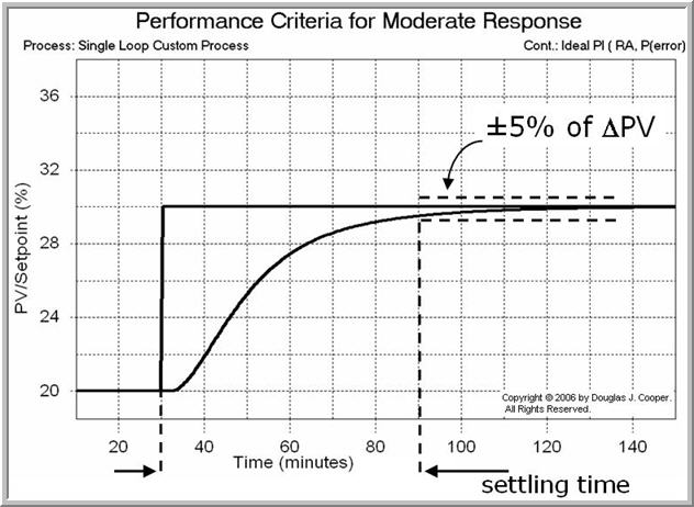
We compute for this plot:
Settling Time = (90 – 30) = 60 min for a ±5% of DPV band
Isn’t it interesting that a more moderately tuned controller has a faster settling time then the more active or aggressive response shown previously where settling time was 70 minutes? (In truth, this is not a surprising result because for the previous plots, the controller was deliberately mistuned to provide the sharp peaks we needed to clearly illustrate the performance definitions.)
Settling Band is Application Specific
Measurement noise, or random error in the PV signal, can be one reason to modify the width of the settling band. As shown below (click for a larger view), for the identical process and tuning as used in the above moderate response plot, but with significant noise added to the PV, the settling band must to be widened considerably to provide a meaningful measure.
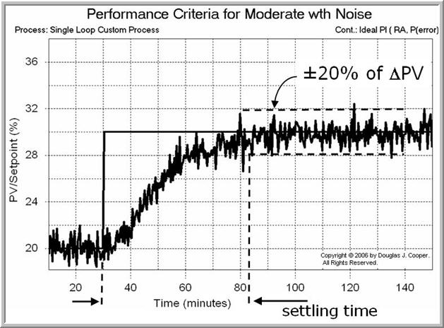
Widening the band in this case is not a bad thing. It is simply necessary. And since we will (presumably) use the same settling band criteria when exploring alternatives for this loop, then it remains a useful tool for comparing performance.
Other Measures
The methods discussed in this article use data from a set response plot to make decisions about the performance of a specific loop in our plant. The methods require some judgment and we must be sure to be consistent for our evaluations to have value.
There are other performance tools and measures that require software to compute. These include moving average, moving variance, cross and auto correlation, power spectrum and more. These will be discussed in a future article.